
Differentiable Illumination Optimization#
NSQ as a differentiable machine-learning layer.
When Optiland’s backend is set to "torch" the non-sequential tracer builds a full PyTorch autograd graph through the Monte Carlo loop. Any scene parameter stored as a torch.Tensor leaf variable — radius of curvature, source flux, BSDF reflectance — receives a gradient via loss.backward().
This notebook walks through a complete differentiable optimization example:
Scene setup — collimated source → singlet lens → irradiance detector
Forward trace — visualize the baseline irradiance map
Optimization loop — use
torch.optim.Adamto drive the lens front radiusr1toward a flat (uniform) irradiance targetResults — loss curve and final irradiance map
Bonus — a second, genuinely new differentiable parameter:
scatter_fractionLimitations — what gradients are and are not available today
Pre-release.
optiland.nonsequentialhas never shipped in a tagged Optiland release, so its public API may still change without a deprecation cycle. The differentiable workflow shown here is fully supported; visibility gradients (silhouette / vignetting discontinuities) are zero (see Section 6). See the roadmap in the package docstring (help(optiland.nonsequential)) for planned improvements.
0. Imports and backend selection#
[1]:
import matplotlib.pyplot as plt
import numpy as np
import torch
import torch.optim as optim

import optiland.backend as be
from optiland.coordinate_system import CoordinateSystem
from optiland.nonsequential import (
    CollimatedSourceConfig,
    IrradianceDetectorConfig,
    LensConfig,
    NSQScene,
    Spectrum,
)
from optiland.nonsequential.backends.torch_backend import TorchBackend

# Switch to the PyTorch backend -- this is required for autograd.
# All optiland.backend operations now use torch under the hood.
be.set_backend("torch")
# Use float64 for gradient stability. The differentiable Monte Carlo trace is
# numerically delicate near surface edges; float64 keeps gradients well-behaved
# at the CPU-runnable ray counts used here.
be.set_precision("float64")

print(f"Backend : {be.get_backend()}")
print(f"Device  : {torch.device('cuda' if torch.cuda.is_available() else 'cpu')}")
Backend : torch
Device  : cuda
1. Scene setup#
We build a simple on-axis system:
Collimated source  →  N-BK7 singlet  →  Irradiance detector
    z = 0              z = 100 mm           z = 210 mm
The singlet has a plano-convex shape (r1 = 120 mm, r2 = inf) and a 10 mm semi-aperture. At z = 210 mm the beam is still converging, so the irradiance map shows a bright central peak — far from uniform.
The detector is 20 × 20 mm with 32 × 32 pixels — small enough to keep memory low during the optimization loop.
[2]:
NUM_PIXELS = 32          # detector resolution (NxN)
DETECTOR_SIZE = 20.0     # mm
SEED = 42


def build_scene(
    r1_value: float | torch.Tensor,
    num_rays: int = 2_000,
) -> NSQScene:
    """Return an NSQScene with a singlet whose front radius is r1_value.

    r1_value may be a plain float (forward-only) or a torch.Tensor with
    requires_grad=True (differentiable).
    """
    spec = Spectrum.monochromatic(0.55)   # 550 nm green

    scene = NSQScene()

    # Collimated beam: 10 mm aperture radius, 1 W total flux
    scene.add_source(
        "S1",
        CoordinateSystem(z=0.0),
        CollimatedSourceConfig(
            spectrum=spec,
            total_flux=1.0,
            aperture_radius=10.0,
        ),
    )

    # Singlet lens: initial r1 = 120 mm, back flat, 5 mm thick N-BK7
    scene.add_lens(
        "L1",
        CoordinateSystem(z=100.0),
        LensConfig(
            r1=r1_value,       # float, or a requires_grad tensor
            r2=float("inf"),   # flat back surface
            thickness=5.0,
            material="N-BK7",
            front_aperture_radius=10.0,
        ),
    )

    # Irradiance detector: 20x20 mm, 32x32 pixels, bilinear splat
    scene.add_detector(
        "D1",
        CoordinateSystem(z=210.0),
        IrradianceDetectorConfig(
            width=DETECTOR_SIZE,
            height=DETECTOR_SIZE,
            num_pixels_x=NUM_PIXELS,
            num_pixels_y=NUM_PIXELS,
            splat="bilinear",   # differentiable splatting
        ),
    )

    return scene


print("Scene factory defined.")
Scene factory defined.
2. Forward trace — baseline irradiance map#
Before optimizing, let’s see what the irradiance pattern looks like with the initial radius r1 = 120 mm. We use a larger ray count here for a clean visualization.
[3]:
with torch.no_grad():
    scene_init = build_scene(r1_value=120.0, num_rays=10_000)
    backend_init = TorchBackend(seed=SEED)
    result_init = backend_init.trace(scene_init, num_rays=10_000, max_depth=8)

irr_init = result_init.detectors["D1"].irradiance   # (ny, nx) numpy array

fig, axes = plt.subplots(1, 2, figsize=(11, 4))

im = axes[0].imshow(
    irr_init, origin="lower",
    extent=[-DETECTOR_SIZE/2, DETECTOR_SIZE/2,
            -DETECTOR_SIZE/2, DETECTOR_SIZE/2],
    cmap="hot",
)
axes[0].set_title("Baseline irradiance (r1 = 120 mm)")
axes[0].set_xlabel("x [mm]")
axes[0].set_ylabel("y [mm]")
plt.colorbar(im, ax=axes[0], label="Irradiance [W/mm²]")

# Cross-section
cy = NUM_PIXELS // 2
axes[1].plot(np.linspace(-DETECTOR_SIZE/2, DETECTOR_SIZE/2, NUM_PIXELS),
             irr_init[cy, :], lw=1.5)
axes[1].set_xlabel("x [mm]")
axes[1].set_ylabel("Irradiance [W/mm²]")
axes[1].set_title("Horizontal cross-section (y = 0)")
axes[1].grid(True, alpha=0.35)

plt.tight_layout()
plt.show()

print(f"Peak irradiance : {irr_init.max():.4f} W/mm²")
print(f"Mean irradiance : {irr_init.mean():.4f} W/mm²")
print(f"Uniformity ratio: {irr_init.mean()/irr_init.max():.3f}  (1.0 = perfect flat top)")
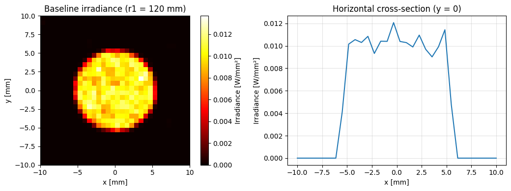
Peak irradiance : 0.0137 W/mm²
Mean irradiance : 0.0023 W/mm²
Uniformity ratio: 0.167  (1.0 = perfect flat top)
3. Optimization loop#
Objective: minimize the mean-squared error (MSE) between the irradiance map and a flat (uniform) target.
Design variable: the front radius of curvature r1 of the singlet.
Gradient path: r1 (a torch.Tensor leaf) → ConicGeometry._sag() → ray_intersect() → refracted direction → splat weight → IrradianceMap.data → loss.backward() → r1.grad.
Ray count note#
We use 2 000 rays per step. This keeps each forward pass fast and keeps memory within the gradient-mode envelope (~1 × 10⁵ rays × depth 16 on a single GPU). Monte Carlo noise at 2 000 rays is noticeable — increase to 10 000–50 000 rays for production runs, at proportionally higher memory cost. Common-random-numbers (fixed seed) reduce variance further.
What loss.backward() does#
PyTorch walks the autograd graph from loss back to r1, accumulating ∂loss/∂r1. optimizer.step() then nudges r1 in the gradient-descent direction. No hand-written Jacobians are needed.
⚠ Visibility gradients are zero. This loop optimizes r1 through the interior refraction path, which is fully differentiable. But if r1 changes enough that rays begin to vignette at an aperture edge, that silhouette boundary contributes no gradient — the single biggest physics gap in this pre-release. Keep design moves within the unvignetted regime, or expect the optimizer to ignore edge effects. See the canonical NSQ Limitations & Roadmap
page (roadmap item #1: reparameterization).
[4]:
NUM_RAYS_OPT  = 2_000    # rays per optimization step
NUM_STEPS     = 60       # Adam steps
LEARNING_RATE = 5.0      # mm / step  (large because radius is in mm)
OPT_SEED      = 7        # fixed seed -> common random numbers

# IrradianceMap.data is the attached flat (ny*nx,) flux buffer. Dividing the
# reshaped grid by the pixel area gives a differentiable irradiance [W/mm^2],
# matching the units of irr_init used to build the target.
PIXEL_AREA = (DETECTOR_SIZE / NUM_PIXELS) ** 2

# ---- design variable -------------------------------------------------------
r1 = torch.tensor(120.0, requires_grad=True, dtype=torch.float64)
optimizer = optim.Adam([r1], lr=LEARNING_RATE)

# ---- flat target irradiance (uniform, same mean) --------------------------
target_value = float(irr_init.mean())   # W/mm^2
target = torch.full(
    (NUM_PIXELS, NUM_PIXELS), target_value, dtype=torch.float64
)

print(f"Target irradiance (flat): {target_value:.5f} W/mm^2")
print(f"Starting r1             : {r1.item():.2f} mm")
print(f"Optimizing for {NUM_STEPS} steps ...")

# ---- optimization loop -----------------------------------------------------
loss_history = []
r1_history   = []

for step in range(NUM_STEPS):
    optimizer.zero_grad()

    # Rebuild the scene each step so the tensor r1 is wired into fresh geometry.
    # This is the standard pattern for NSQ differentiable optimization.
    scene = build_scene(r1_value=r1, num_rays=NUM_RAYS_OPT)
    backend = TorchBackend(seed=OPT_SEED)   # same seed -> low-variance gradient
    result = backend.trace(scene, num_rays=NUM_RAYS_OPT, max_depth=8)

    # Differentiable irradiance map [W/mm^2] (grad_fn attached)
    irr_tensor = (
        result.detectors["D1"].data.reshape(NUM_PIXELS, NUM_PIXELS) / PIXEL_AREA
    )

    # MSE vs. flat target
    loss = torch.mean((irr_tensor - target) ** 2)

    # Backpropagate through the entire Monte Carlo trace
    loss.backward()

    # Clip gradient to stabilise early steps
    torch.nn.utils.clip_grad_norm_([r1], max_norm=50.0)

    optimizer.step()

    # Clamp to a physically sensible range (avoid near-zero or negative radius)
    with torch.no_grad():
        r1.clamp_(min=30.0, max=600.0)

    loss_history.append(loss.item())
    r1_history.append(r1.item())

    if (step + 1) % 10 == 0:
        print(
            f"Step {step+1:3d}/{NUM_STEPS}  "
            f"loss={loss.item():.2e}  "
            f"r1={r1.item():.2f} mm  "
            f"grad={r1.grad.item():.3e}"
        )

print(f"\nFinal r1 = {r1.item():.2f} mm  (started at 120.00 mm)")
Target irradiance (flat): 0.00229 W/mm^2
Starting r1             : 120.00 mm
Optimizing for 60 steps ...
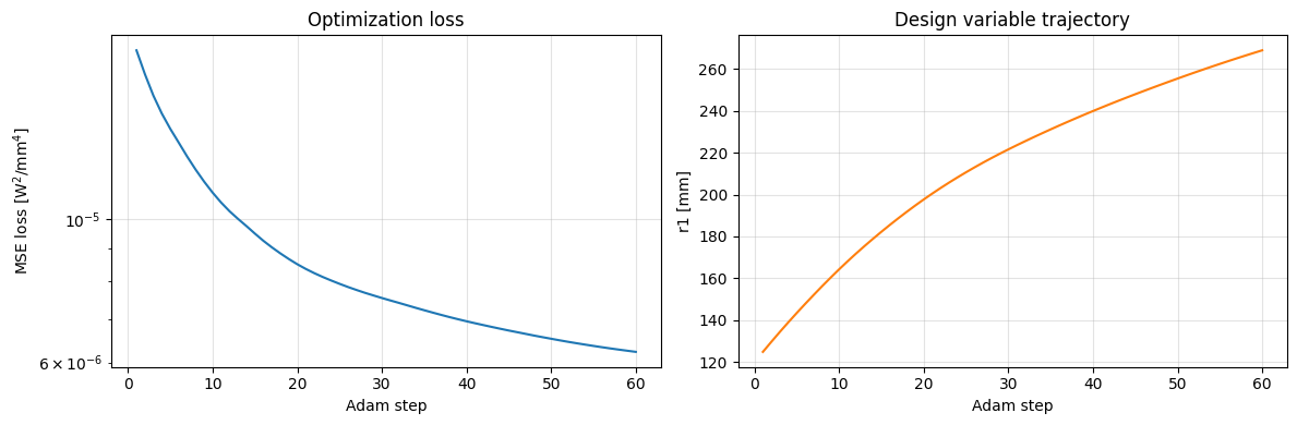
Step  10/60  loss=1.10e-05  r1=164.26 mm  grad=-1.023e-07
Step  20/60  loss=8.51e-06  r1=197.64 mm  grad=-5.093e-08
Step  30/60  loss=7.55e-06  r1=221.56 mm  grad=-3.236e-08
Step  40/60  loss=6.95e-06  r1=239.87 mm  grad=-2.907e-08
Step  50/60  loss=6.53e-06  r1=255.39 mm  grad=-2.505e-08
Step  60/60  loss=6.23e-06  r1=268.88 mm  grad=-1.938e-08

Final r1 = 268.88 mm  (started at 120.00 mm)
4. Results — loss curve and final irradiance map#
[5]:
fig, axes = plt.subplots(1, 2, figsize=(12, 4))

# ---- loss curve ----
ax = axes[0]
ax.semilogy(range(1, NUM_STEPS + 1), loss_history, lw=1.5, color="tab:blue")
ax.set_xlabel("Adam step")
ax.set_ylabel("MSE loss [W$^2$/mm$^4$]")
ax.set_title("Optimization loss")
ax.grid(True, alpha=0.35)

# ---- r1 trajectory ----
ax = axes[1]
ax.plot(range(1, NUM_STEPS + 1), r1_history, lw=1.5, color="tab:orange")
ax.set_xlabel("Adam step")
ax.set_ylabel("r1 [mm]")
ax.set_title("Design variable trajectory")
ax.grid(True, alpha=0.35)

plt.tight_layout()
plt.show()
[6]:
# ---- final irradiance map (higher ray count for cleaner visualization) ----
with torch.no_grad():
    scene_final = build_scene(r1_value=r1.item(), num_rays=20_000)
    backend_final = TorchBackend(seed=SEED)
    result_final = backend_final.trace(scene_final, num_rays=20_000, max_depth=8)

irr_final = result_final.detectors["D1"].irradiance

# Use a shared colour scale so both maps are directly comparable
vmax = max(irr_init.max(), irr_final.max())

fig, axes = plt.subplots(1, 2, figsize=(12, 4.5))
extent = [-DETECTOR_SIZE/2, DETECTOR_SIZE/2,
          -DETECTOR_SIZE/2, DETECTOR_SIZE/2]

for ax, irr, title in zip(
    axes,
    [irr_init, irr_final],
    [f"Before  (r1 = 120.00 mm)",
     f"After   (r1 = {r1.item():.1f} mm)"],
):
    im = ax.imshow(irr, origin="lower", extent=extent,
                   cmap="hot", vmin=0, vmax=vmax)
    ax.set_title(title)
    ax.set_xlabel("x [mm]")
    ax.set_ylabel("y [mm]")
    plt.colorbar(im, ax=ax, label="Irradiance [W/mm²]")

plt.suptitle("Differentiable irradiance optimization", fontsize=13)
plt.tight_layout()
plt.show()

uniformity_before = irr_init.mean() / (irr_init.max() + 1e-12)
uniformity_after  = irr_final.mean() / (irr_final.max() + 1e-12)
print(f"Uniformity ratio before : {uniformity_before:.3f}")
print(f"Uniformity ratio after  : {uniformity_after:.3f}")
print(f"(1.0 = perfectly flat top)")
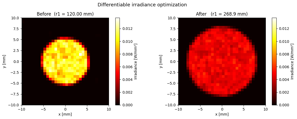
Uniformity ratio before : 0.167
Uniformity ratio after  : 0.367
(1.0 = perfectly flat top)
5. Bonus: gradients through scatter_fraction#
Lens radius is not the only newly-expanded gradient path. BSDF parameters — including a surface’s scatter_fraction, the probability that a hit ray is routed through a scatter model (LambertianBSDF, HarveyShackBSDF, …) instead of following its specular/refractive path — are now differentiable too. Previously this branch was sampled but the weight was not attached to scatter_fraction, so ∂loss/∂scatter_fraction was silently zero; it now uses the same
detached-sample/attached-weight estimator as the Fresnel split, so the gradient is correct rather than dead.
To show this cleanly, build a tiny standalone scene: a flat diffusing plate on-axis, with an off-axis detector that can only receive flux that scattered (the unscattered beam continues straight through and misses it entirely). If scatter_fraction carries a gradient, ∂(side detector flux)/∂(scatter_fraction) should be positive and finite — more scattering, more flux reaches the side detector.
[7]:
from optiland.nonsequential import RefractiveComponent, NSQMaterial, VACUUM, LambertianBSDF
from optiland.nonsequential.components.geometry.analytic.plane import FinitePlaneGeometry

# scatter_fraction as a differentiable leaf.
sf = torch.tensor(0.3, requires_grad=True, dtype=torch.float64)

diffuser = RefractiveComponent(
    cs=CoordinateSystem(z=50.0),
    geometry=FinitePlaneGeometry(width=30, height=30),
    material_front=VACUUM,
    material_back=NSQMaterial.from_glass("N-BK7"),
    bsdf=LambertianBSDF(reflectance_value=1.0),   # fully reflective when scattered
    scatter_fraction=sf,
    name="diffuser",
)

scene_sf = NSQScene()
scene_sf.add_source(
    "S1", CoordinateSystem(z=0.0),
    CollimatedSourceConfig(spectrum=Spectrum.monochromatic(0.55),
                           total_flux=1.0, aperture_radius=8.0),
)
scene_sf.add_component("diffuser", diffuser)
# Off-axis, facing the diffuser: the specular (unscattered) beam travels
# straight ahead and cannot hit this detector -- everything it records
# arrived via the Lambertian scatter branch.
scene_sf.add_detector(
    "side", CoordinateSystem(x=15, z=50, ry=np.pi / 2),
    IrradianceDetectorConfig(width=40, height=40, num_pixels_x=16, num_pixels_y=16,
                             splat="bilinear"),
)

backend_sf = TorchBackend(seed=3)
result_sf = backend_sf.trace(scene_sf, num_rays=8_000, max_depth=4)
side_flux = result_sf.detectors["side"].data.sum()   # attached, differentiable
side_flux.backward()

print(f"scatter_fraction        : {sf.item():.3f}")
print(f"Side-detector flux      : {side_flux.item():.5f} W  (only reachable via scatter)")
print(f"d(side flux)/d(scatter_fraction) : {sf.grad.item():.4f}")
print("\nPositive and finite: more scattering sends measurably more flux "
      "sideways, and the gradient says so directly -- no finite differences "
      "needed.")
scatter_fraction        : 0.300
Side-detector flux      : 0.05437 W  (only reachable via scatter)
d(side flux)/d(scatter_fraction) : 0.1813

Positive and finite: more scattering sends measurably more flux sideways, and the gradient says so directly -- no finite differences needed.
6. Limitations and how to work around them#
What works#
Pass a torch.tensor(..., requires_grad=True) straight into the ordinary config object — no private attributes, no post-construction patching.
Parameter |
How |
|---|---|
Lens radius ( |
|
Component aperture radius |
|
Mirror radius |
|
Source |
|
BSDF reflectance / transmittance, including |
|
Material refractive index (dispersion-formula glass) |
|
Irradiance detector |
|
Detector pixel counts are integers and structural, so they are not differentiable.
Parameters that cannot carry gradients raise ``NotImplementedError`` rather than detaching silently — a design variable that has no effect on the loss should fail loudly, not sit at zero gradient. This applies to source geometry (aperture_radius, half_angle_deg, extended-source extent), whose sampling runs in NumPy, and to SpectralDetector extents.
What does NOT work today#
Visibility gradients are zero. When
r1is changed enough that rays start to vignette at the aperture edge, the gradient through that boundary is zero. The optimizer can still make progress through the interior (refraction) path, but the silhouette contribution is missing. Roadmap item #1 — reparameterization — will fix this.Mesh geometry is forward-only.
MeshGeometry.ray_intersect()uses a numpy BVH; callingloss.backward()through it will raise. UseConicGeometry/SphereGeometry/ParaboloidGeometryfor differentiable surfaces.Memory cap at ~1 × 10⁵ rays. The fixed-depth autograd graph stores O(num_rays × max_depth) activations. At 2 000 rays and depth 8 the footprint is negligible; at 1 × 10⁵ rays and depth 16 you will need ~8 GB of GPU VRAM. Roadmap item #3 — Path Replay Backpropagation — reduces this to O(num_rays).
No polarization. Stokes tracking is on the roadmap.
Tips for stable optimization#
Common-random-numbers (fixed seed): re-using the same RNG seed across steps keeps gradient variance low (as done above with
OPT_SEED = 7).Gradient clipping:
clip_grad_norm_prevents large steps early in training when the gradient is noisy.Warm start: run 5–10 forward-only passes first to verify the scene produces rays on the detector before enabling autograd.
Detach for diagnostics: wrap visualization/metrics in
with torch.no_grad():to avoid building unnecessary graph nodes.
Summary#
The minimum differentiable NSQ loop is:
import optiland.backend as be
import torch, torch.optim as optim
from optiland.nonsequential.backends.torch_backend import TorchBackend

be.set_backend("torch")
be.set_precision("float64")   # recommended for gradient work

r1 = torch.tensor(120.0, requires_grad=True, dtype=torch.float64)
optimizer = optim.Adam([r1], lr=5.0)

for step in range(100):
    optimizer.zero_grad()
    scene = build_scene(r1)           # LensConfig(r1=r1) - tensor goes straight in
    result = TorchBackend(seed=42).trace(scene, num_rays=2_000)
    loss = my_loss(result.detectors["D1"].data)
    loss.backward()                   # gradient through full MC trace
    optimizer.step()
Feedback and contributions welcome. If you use this workflow for a real illumination or stray-light problem, open a GitHub issue and describe your use case — feedback directly shapes the roadmap: HarrisonKramer/optiland#issues