Getting Started with Non-Sequential Ray Tracing

This notebook introduces the core workflow of the Optiland non-sequential (NSQ) ray tracer. In sequential ray tracing, rays travel through surfaces in a fixed order. In non-sequential tracing, rays propagate freely through a scene, bouncing, refracting, and scattering on any surface they encounter, in any order.

This makes NSQ tracing ideal for:

• Illumination design and uniformity analysis

• Stray light and ghost image analysis

• Scatter and diffuse surface modeling

• Non-imaging optics (concentrators, light pipes)

By the end of this notebook you will know how to:

1. Create an NSQScene and populate it with a source, a lens, and a detector

2. Run a Monte Carlo ray trace

3. Inspect the SimulationResult and visualize the irradiance map

import matplotlib.pyplot as plt
import numpy as np

from optiland.coordinate_system import CoordinateSystem
from optiland.nonsequential import (
    NSQScene,
    Spectrum,
    PointSourceConfig,
    LensConfig,
    IrradianceDetectorConfig,
)

1. Describing a Wavelength with Spectrum

Every NSQ source needs a Spectrum — a probability distribution over wavelengths (in micrometres). The simplest case is monochromatic light:

# 550 nm = 0.55 µm — green light
spec = Spectrum.monochromatic(0.55)
print(f"Wavelength: {spec.wavelengths[0]:.3f} µm")

Wavelength: 0.550 µm

2. Building the Scene

An NSQScene contains three kinds of objects:

• Sources — emit rays into the scene

• Components — optical elements that redirect rays (lenses, mirrors)

• Detectors — record rays that hit them

Each object has a ``CoordinateSystem`` that defines its position and orientation. All coordinates are in millimetres; rotations rx, ry, rz are in radians.

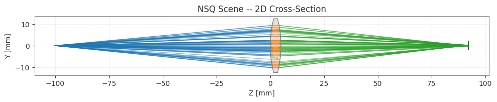
Here we set up a simple system:

Point source  →  Biconvex lens  →  Irradiance detector
   z = -100         z = 0              z = 92

Two choices in that layout are worth spelling out, because getting either wrong is the most common way a first NSQ scene produces a meaningless picture.

The source has to fit the lens. A point source 100 mm from a lens with a 12.5 mm semi-diameter fills the aperture at atan(12.5/100) = 7.1°. Ask for a wider cone and the surplus rays sail straight past the glass to the detector, where they swamp the image with light that never went through the lens. We use 6°, which underfills the aperture slightly.

The detector has to be at the image. This lens has f = 49.1 mm, so an object 100 mm in front of it images to roughly 96 mm behind it. Spherical aberration pulls the tightest spot slightly inside that, to about z = 92 mm. Put the detector at, say, z = 200 mm instead and you measure a defocus blur.

scene = NSQScene()

# --- Source -----------------------------------------------------------------
# PointSource at z = -100 mm, emitting a 6-degree cone toward +z. At 100 mm
# that is a 10.5 mm beam radius, just inside the lens semi-diameter of 12.5 mm.
scene.add_source(
    'S1',
    CoordinateSystem(z=-100),
    PointSourceConfig(spectrum=spec, total_flux=1.0, half_angle_deg=6.0),
)

# --- Lens -------------------------------------------------------------------
# Biconvex N-BK7 lens at z = 0 mm
# r1 = 50 mm (front), r2 = -50 mm (back), center thickness = 5 mm
# semi-diameter = 12.5 mm
scene.add_lens(
    'L1',
    CoordinateSystem(z=0),
    LensConfig(r1=50, r2=-50, thickness=5, material='N-BK7', front_aperture_radius=12.5),
)

# --- Detector ---------------------------------------------------------------
# 4 x 4 mm irradiance detector at the image plane. Sized to the spot, not to
# the lens: the image is a few tenths of a millimetre across, so a 20 mm
# detector would spend 128 pixels resolving mostly empty space.
scene.add_detector(
    'D1',
    CoordinateSystem(z=92),
    IrradianceDetectorConfig(width=4, height=4, num_pixels_x=128, num_pixels_y=128),
)

print("Scene components:", scene.component_names)
print("Sources         :", scene.source_names)
print("Detectors       :", scene.detector_names)

Scene components: ['L1']
Sources         : ['S1']
Detectors       : ['D1']

View the current scene

scene.view() draws a cross-section through the scene and overlays a sample of traced rays. color_by='bounce' gives each leg of a ray path its own colour, so you can see the beam enter the glass, leave it, and converge on the detector — the non-sequential path, rather than a surface-by-surface list.

scene.view(num_rays=80, color_by='bounce')
plt.show()

3. Running the Monte Carlo Trace

scene.trace() launches the simulation. Key parameters:

Parameter	Meaning	Default
num_rays	Total rays launched	—
max_depth	Maximum surface hits per ray	16
min_flux_fraction	Russian-roulette threshold, relative to a ray’s initial flux: below it a ray is killed with an unbiased probability and survivors’ flux is boosted to compensate, rather than being truncated outright	1e-6
seed	RNG seed for reproducibility	None

A SimulationResult is returned with per-detector results and global statistics.

result = scene.trace(num_rays=100_000, seed=42)
print(f"Trace time          : {result.trace_time_sec:.2f} s")
print(f"Rays launched       : {result.num_rays_total:,}")
print(f"Rays on detector    : {result.detectors['D1'].num_rays_hit:,}")
print(f"Total flux in       : {result.total_flux_in:.4f} W")
print(f"Flux on detector    : {result.total_flux_detected:.4f} W")
print(f"Flux escaped        : {result.total_flux_escaped:.4f} W")
print(f"Flux conservation   : {result.flux_conservation_error:.2e} (relative error)")
print()
print("Most of the launched flux escapes: the source emits into a 6-degree cone")
print("but the detector is only 4 mm across, so it collects the image and")
print("nothing else. Flux conservation is the number to check, not the fraction")
print("landing on any one detector.")

Trace time          : 0.38 s
Rays launched       : 100,000
Rays on detector    : 91,712
Total flux in       : 1.0000 W
Flux on detector    : 0.9165 W
Flux escaped        : 0.0828 W
Flux conservation   : 8.33e-17 (relative error)

Most of the launched flux escapes: the source emits into a 6-degree cone
but the detector is only 4 mm across, so it collects the image and
nothing else. Flux conservation is the number to check, not the fraction
landing on any one detector.

result.report() — read this first

Every SimulationResult carries a diagnostics object that catches the failure modes that would otherwise show up as a silently wrong-looking plot: rays killed by the max_depth cap before they resolved, flux lost to Russian-roulette termination, scene geometry no ray ever reached, and detectors sampled too sparsely to trust. result.report() prints all of it with threshold-based warnings — running it is the first thing to do after every trace, before looking at any plot.

print(result.report())

NSQ trace diagnostics:
  depth_truncated_flux_fraction: 0.0000%
  rr_killed_flux_fraction:       0.0000%
  flux_conservation_error:       0.0000%
  unreached_geometry:            ['L1.edge']
  medium_stack_underflows:       0
  split_budget_saturated:        False
  detectors:
    D1: 91712 hits, 5.60 mean hits/pixel [undersampled]
Warnings:
  - 1 component(s) were never hit by any ray: L1.edge. Check placement/orientation, or ignore if intentionally unused.
  - Detector 'D1' is undersampled: 5.6 mean hits/pixel (< 10), shot noise dominates the map; ~7,145,847 rays would bring it to ~5% relative error.

Two warnings show up here, and both are expected for this particular scene rather than something to fix:

• ``L1.edge`` unreached — the lens edge (its cylindrical barrel) is only hit by rays wide enough to miss both curved faces. A 6° cone underfilling a 12.5 mm aperture never comes close, so the edge going unused is exactly what should happen. If a curved face were reported unreached, that would mean the beam is missing the lens.

• ``D1`` undersampled (5.6 mean hits/pixel) — 100,000 rays spread over a 128×128 grid is a deliberately small trace for a fast-running tutorial; report() estimates the ~7 million rays a production-quality, low-noise map would need. Scale num_rays up for a publication-quality figure.

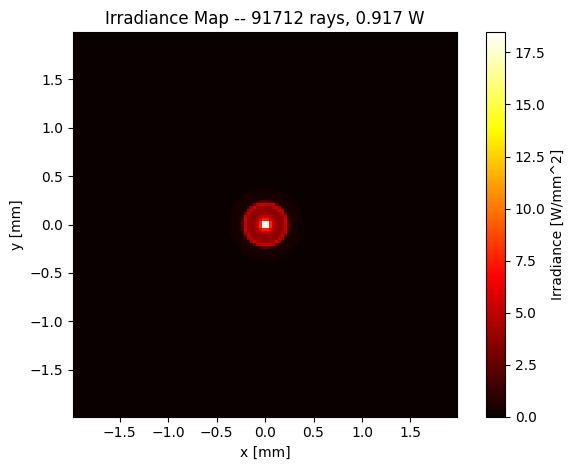
4. Visualizing the Irradiance Map

Each detector in result.detectors holds a result object. For an IrradianceDetector the result is an IrradianceMap with a .plot() method.

irr_map = result.detectors['D1']

fig = irr_map.plot(cmap='hot')
plt.tight_layout()
plt.show()

5. Inspecting the Raw Irradiance Array

IrradianceMap.irradiance is a 2-D NumPy array of shape (ny, nx) in W/mm². You can compute statistics directly:

E = irr_map.irradiance
print(f"Array shape    : {E.shape}")
print(f"Peak irradiance: {E.max():.4f} W/mm²")
print(f"Mean irradiance: {E.mean():.6f} W/mm²")
print(f"Total flux     : {irr_map.total_flux:.4f} W")

Array shape    : (128, 128)
Peak irradiance: 18.4647 W/mm²
Mean irradiance: 0.057283 W/mm²
Total flux     : 0.9165 W

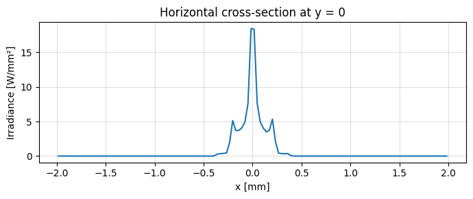
6. Cross-Section Plot

Take a horizontal slice through the centre of the irradiance map:

ny, nx = E.shape
centre_row = E[ny // 2, :]

fig, ax = plt.subplots(figsize=(7, 3))
ax.plot(irr_map.x_coords, centre_row)
ax.set_xlabel('x [mm]')
ax.set_ylabel('Irradiance [W/mm²]')
ax.set_title('Horizontal cross-section at y = 0')
ax.grid(True, alpha=0.4)
plt.tight_layout()
plt.show()

Summary

The minimum NSQ workflow is:

scene = NSQScene()
scene.add_source(name, cs, SourceConfig(...))
scene.add_lens(name, cs, LensConfig(...))
scene.add_detector(name, cs, DetectorConfig(...))
result = scene.trace(num_rays=N, seed=42)
print(result.report())          # check for warnings before trusting the plot
result.detectors[name].plot()

Continue to the next notebooks to learn about the different source types, component options, detectors, and advanced features.