Ray Sources

The NSQ engine provides three source types that cover most real-world scenarios:

Class	Geometry	Typical use
PointSource	Single point, cone emission	LED die, lamp filament
CollimatedSource	Circular disk, parallel rays	Laser beam, far-field source
ExtendedSource	Rectangular or circular area, cone or cosine emission	Display panel, diffuse emitter

All sources require a Spectrum object (wavelengths in µm) and accept a total_flux in watts. Their position and orientation are set by a CoordinateSystem.

import matplotlib.pyplot as plt
import numpy as np

from optiland.coordinate_system import CoordinateSystem
from optiland.nonsequential import (
    NSQScene, Spectrum,
    PointSourceConfig, CollimatedSourceConfig, ExtendedSourceConfig,
    IrradianceDetectorConfig, RayDatabaseConfig,
)
from optiland.nonsequential.rng import NSQRng

1. Spectra

Monochromatic spectrum

A single wavelength — the fastest and simplest option:

spec_green = Spectrum.monochromatic(0.55)   # 550 nm
spec_red   = Spectrum.monochromatic(0.633)  # 633 nm HeNe laser
spec_blue  = Spectrum.monochromatic(0.45)   # 450 nm

Broadband spectrum

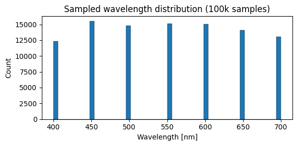
Pass arrays of wavelengths (µm) and relative spectral weights. The weights are normalised internally and used for Monte Carlo sampling — so only their ratios matter, not their absolute values.

Spectrum.sample() draws from a keyed PCG32 RNG (optiland.nonsequential.rng.NSQRng), the same generator the tracer uses internally: every wavelength is a pure function of (seed, ray_id, bounce) rather than of a mutable stream position, which is what makes NSQ results reproducible across batch_size and ray compaction. ray_id is just “which ray” — an arbitrary distinct integer per draw is enough to get independent samples here:

# Rough D65 visible spectrum sampled at 7 wavelengths
spec_white = Spectrum(
    wavelengths=np.array([0.40, 0.45, 0.50, 0.55, 0.60, 0.65, 0.70]),
    weights=np.array([0.82, 1.04, 1.00, 1.01, 1.00, 0.95, 0.88]),
)

# Sample 100k wavelengths from the spectrum and check the distribution.
# ray_id supplies the "which draw" key for the PCG32 RNG; bounce=0 since
# this has nothing to do with an actual trace depth.
rng = NSQRng(seed=0)
ray_id = np.arange(100_000)
samples = spec_white.sample(ray_id, bounce=0, rng=rng)

fig, ax = plt.subplots(figsize=(6, 3))
ax.hist(samples * 1000, bins=50, edgecolor='k', linewidth=0.3)
ax.set_xlabel('Wavelength [nm]')
ax.set_ylabel('Count')
ax.set_title('Sampled wavelength distribution (100k samples)')
plt.tight_layout()
plt.show()

2. PointSource

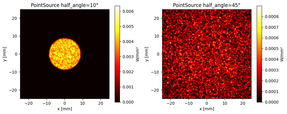
A point emitter with configurable solid-angle cone:

• half_angle_deg=90 → hemisphere (default)

• half_angle_deg=180 → full sphere (isotropic)

• half_angle_deg=<small> → narrow forward cone

The CoordinateSystem controls the cone axis: the source emits along the local +z direction.

def irradiance_from_point_source(half_angle_deg, num_rays=30_000):
    scene = NSQScene()
    scene.add_source(
        'S', CoordinateSystem(z=0),
        PointSourceConfig(spectrum=spec_green, total_flux=1.0,
                          half_angle_deg=half_angle_deg),
    )
    scene.add_detector(
        'D', CoordinateSystem(z=50),
        IrradianceDetectorConfig(width=50, height=50, num_pixels_x=128, num_pixels_y=128),
    )
    result = scene.trace(num_rays=num_rays, seed=0)
    return result.detectors['D']

narrow = irradiance_from_point_source(10)
wide   = irradiance_from_point_source(45)

fig, axes = plt.subplots(1, 2, figsize=(10, 4))
for ax, irr, angle in zip(axes, [narrow, wide], [10, 45]):
    im = ax.imshow(irr.irradiance, origin='lower',
                   extent=[irr.x_coords[0], irr.x_coords[-1],
                            irr.y_coords[0], irr.y_coords[-1]],
                   cmap='hot', aspect='equal')
    plt.colorbar(im, ax=ax, label='W/mm²')
    ax.set_title(f'PointSource half_angle={angle}°')
    ax.set_xlabel('x [mm]'); ax.set_ylabel('y [mm]')
plt.tight_layout()
plt.show()

3. CollimatedSource

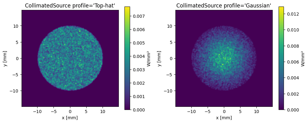
Emits a parallel beam from a circular aperture. Useful for modelling a laser or a distant (infinitely far) source.

Two spatial profiles are available:

• profile='tophat' — uniform irradiance across the beam

• profile='gaussian' — Gaussian irradiance profile

def irradiance_from_collimated(profile, aperture_radius=10, num_rays=30_000):
    scene = NSQScene()
    scene.add_source(
        'S', CoordinateSystem(z=0),
        CollimatedSourceConfig(
            spectrum=spec_green, total_flux=1.0,
            aperture_radius=aperture_radius, profile=profile,
        ),
    )
    scene.add_detector(
        'D', CoordinateSystem(z=50),
        IrradianceDetectorConfig(width=30, height=30, num_pixels_x=128, num_pixels_y=128),
    )
    result = scene.trace(num_rays=num_rays, seed=0)
    return result.detectors['D']

tophat   = irradiance_from_collimated('tophat')
gaussian = irradiance_from_collimated('gaussian')

fig, axes = plt.subplots(1, 2, figsize=(10, 4))
for ax, irr, title in zip(axes, [tophat, gaussian], ['Top-hat', 'Gaussian']):
    im = ax.imshow(irr.irradiance, origin='lower',
                   extent=[irr.x_coords[0], irr.x_coords[-1],
                            irr.y_coords[0], irr.y_coords[-1]],
                   cmap='viridis', aspect='equal')
    plt.colorbar(im, ax=ax, label='W/mm²')
    ax.set_title(f'CollimatedSource profile={title!r}')
    ax.set_xlabel('x [mm]'); ax.set_ylabel('y [mm]')
plt.tight_layout()
plt.show()

4. ExtendedSource

An area emitter. Each ray leaves a random point on the source surface, which is a width x height rectangle by default or a disc when aperture_radius is given.

The emission law depends on half_angle_deg:

• ``half_angle_deg < 90``: rays are spread uniformly over a cone of that half-angle. Use this for a directional emitter.

• ``half_angle_deg >= 90``: rays are cosine-weighted over the full hemisphere, i.e. genuinely Lambertian. Values above 90 behave the same as 90, since the hemisphere is already complete.

Useful for display panels, diffuse luminaires, and, with a small half-angle, the finite angular size of a distant source such as the Sun.

# A 60 deg cone from a 10 x 5 mm rectangle: uniform within the cone
scene = NSQScene()
scene.add_source(
    'S', CoordinateSystem(z=0),
    ExtendedSourceConfig(
        spectrum=spec_green, total_flux=1.0,
        width=10, height=5, half_angle_deg=60,
    ),
)
scene.add_detector(
    'D', CoordinateSystem(z=30),
    IrradianceDetectorConfig(width=40, height=40, num_pixels_x=128, num_pixels_y=128),
)
result = scene.trace(num_rays=50_000, seed=0)
irr_cone = result.detectors['D']

# The same source emitting Lambertian over the full hemisphere
scene_lam = NSQScene()
scene_lam.add_source(
    'S', CoordinateSystem(z=0),
    ExtendedSourceConfig(
        spectrum=spec_green, total_flux=1.0,
        width=10, height=5, half_angle_deg=90,
    ),
)
scene_lam.add_detector(
    'D', CoordinateSystem(z=30),
    IrradianceDetectorConfig(width=40, height=40, num_pixels_x=128, num_pixels_y=128),
)
irr_lam = scene_lam.trace(num_rays=50_000, seed=0).detectors['D']

fig, axes = plt.subplots(1, 2, figsize=(11, 4))
extent = [irr_cone.x_coords[0], irr_cone.x_coords[-1],
          irr_cone.y_coords[0], irr_cone.y_coords[-1]]
for ax, irr, title in zip(
    axes, [irr_cone, irr_lam],
    ['half_angle_deg=60 (uniform cone)', 'half_angle_deg=90 (Lambertian)'],
):
    im = ax.imshow(irr.irradiance, origin='lower', extent=extent, cmap='inferno')
    plt.colorbar(im, ax=ax, label='W/mm$^2$')
    ax.set_title(f'{title}\n{irr.total_flux:.3f} W on detector')
    ax.set_xlabel('x [mm]')
    ax.set_ylabel('y [mm]')
plt.tight_layout()
plt.show()

print(f"60 deg cone : {irr_cone.num_rays_hit:,} rays, {irr_cone.total_flux:.4f} W")
print(f"Lambertian  : {irr_lam.num_rays_hit:,} rays, {irr_lam.total_flux:.4f} W")

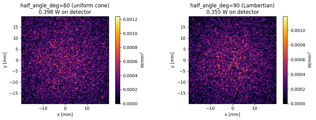
60 deg cone : 19,877 rays, 0.3975 W
Lambertian  : 17,734 rays, 0.3547 W

5. Broadband Source Example

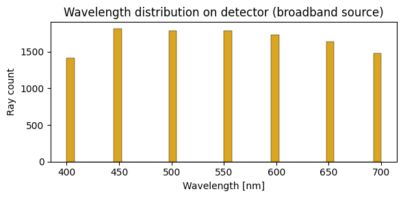
Using the spec_white spectrum defined earlier, launch a broadband point source and verify the wavelength distribution on the detector via a RayDatabaseDetector:

scene2 = NSQScene()
scene2.add_source(
    'S', CoordinateSystem(z=0),
    PointSourceConfig(spectrum=spec_white, total_flux=1.0, half_angle_deg=30),
)

# A RayDatabaseDetector stores every hitting ray as a full phase-space record.
scene2.add_detector(
    'RDB', CoordinateSystem(z=40),
    RayDatabaseConfig(width=30, height=30),
)

result2 = scene2.trace(num_rays=20_000, seed=1)
db = result2.detectors['RDB']

fig, ax = plt.subplots(figsize=(6, 3))
ax.hist(db.wavelength * 1000, bins=40, color='goldenrod', edgecolor='k', linewidth=0.3)
ax.set_xlabel('Wavelength [nm]')
ax.set_ylabel('Ray count')
ax.set_title('Wavelength distribution on detector (broadband source)')
plt.tight_layout()
plt.show()

Summary

• All wavelengths are in µm throughout the NSQ engine

• Spectrum.monochromatic(wl_um) for single-wavelength simulations

• Spectrum(wavelengths, weights) for polychromatic simulations

• PointSource — cone emitter; half_angle_deg controls the beam spread

• CollimatedSource — parallel beam; aperture_radius sets the beam size

• ExtendedSource — area emitter; a uniform cone below 90 deg half-angle, cosine-weighted (Lambertian) at 90 deg and above

• Multiple sources can be added to a single scene