Non-Sequential Ray Tracing#

The Optiland non-sequential (NSQ) engine is a Monte Carlo ray tracer for illumination design, stray light analysis, and non-imaging optics. Unlike the sequential tracer — where surfaces are numbered and rays always traverse them in order — the NSQ engine lets rays propagate freely through a 3-D scene, bouncing, refracting, and scattering on any surface they encounter.

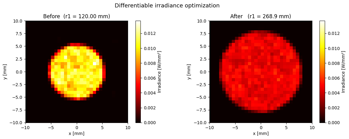
Two engines, two jobs. NSQ runs forward on NumPy (1e7+ rays — the real illumination and stray-light workflow) and differentiably on PyTorch (be.set_backend("torch"), ~1e5 rays at depth 16 — optimization and ML layers). The same scene-building code drives both; switching the active optiland.backend selects the engine. The forward path is for production analysis; the torch path builds a full autograd graph through the Monte Carlo loop so you can shape a detector’s irradiance by calling loss.backward() (see notebook 11).

Already have a lens? Convert it in one line. Existing sequential Optiland designs drop straight into NSQ for stray-light and ghost analysis:

from optiland.nonsequential import sequential_to_nonsequential
scene = sequential_to_nonsequential(optic)   # singlets → Lens, doublets → Doublet, image → IrradianceDetector

Note

Pre-release. NSQ has never shipped in a tagged Optiland release, so the API may still change without a deprecation cycle. See NSQ Limitations & Roadmap (canonical) for the capability envelope, known limitations (notably zero visibility gradients), and the development roadmap. See NSQ Validation Report for the closed-form benchmarks and invariants the engine is checked against in CI.

When to use the NSQ engine

Illumination design — uniform lighting, LED arrays, light-pipe uniformity
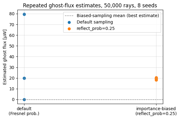
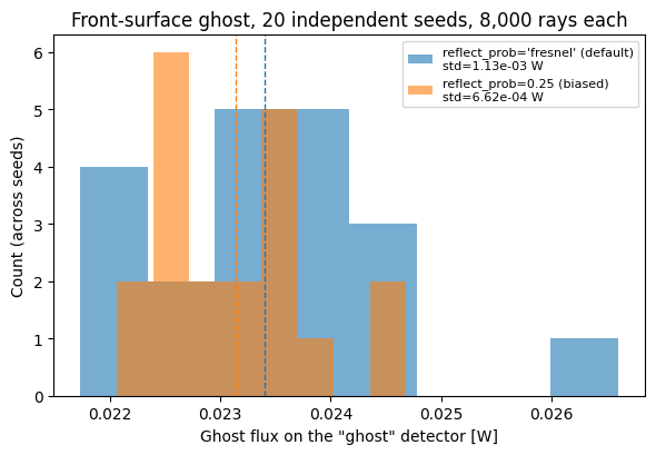
Stray light / ghost analysis — Fresnel reflections, inter-lens ghosts
Scatter modelling — diffuse coatings, rough mirrors (Harvey–Shack ABg model)
Non-imaging optics — solar concentrators, parabolic reflectors
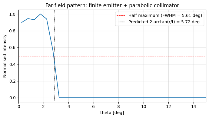
Detector characterisation — encircled energy, spot diagrams, far-field patterns

Sequential vs. non-sequential

Use the sequential engine for imaging design (lenses in a known order, one image plane, deterministic ray tracing). Reach for NSQ when light order is not fixed or when you care about where stray light lands.

	Sequential	Non-sequential (NSQ)
Propagation	Ordered surface list	Free 3-D propagation, any order
Typical job	Imaging / aberration design	Illumination, stray light, non-imaging
Targets	One image surface	Many detectors anywhere in the scene
Method	Deterministic ray trace	Monte Carlo sampling
Splitting	Single path per ray	Fresnel reflect/refract, scatter, ghosts

Core concepts

NSQScene: The central container. Holds sources, compound components (lenses, mirrors, doublets), and detectors. Call scene.trace(num_rays=N) to run the simulation and receive a SimulationResult.
Coordinate system: Every object (source, component, detector) is placed with a CoordinateSystem. Positions are in mm; rotation angles rx, ry, rz are in radians.
Spectrum: All wavelengths in the NSQ engine are in micrometres (µm). Use Spectrum.monochromatic(wl_um) for a single wavelength or Spectrum(wavelengths, weights) for a polychromatic distribution.

Sources

Class	Config	Description
`PointSource`	`PointSourceConfig`	Single point; configurable emission cone (`half_angle_deg`)
`CollimatedSource`	`CollimatedSourceConfig`	Parallel beam; `tophat` or `gaussian` spatial profile
`ExtendedSource`	`ExtendedSourceConfig`	Rectangular Lambertian emitter; width × height

Components

Class	Config	Description
`Lens`	`LensConfig`	Single refractive element; Fresnel splitting at each face
`Doublet`	`DoubletConfig`	Cemented achromatic doublet; crown + flint elements
`Mirror`	`MirrorConfig`	Conic reflective surface; conic=0 (sphere), -1 (paraboloid). `reflectance` is required — a constant, a wavelength-dependent callable, or a coating; there is no implicit perfect-mirror default.

Detectors

Class	Config	Result class
`IrradianceDetector`	`IrradianceDetectorConfig`	`IrradianceMap` — 2-D spatial flux map [W/mm²]
`FarFieldDetector`	`FarFieldDetectorConfig`	`FarFieldPattern` — angular (θ, φ) intensity [W/sr]
`SpectralDetector`	`SpectralDetectorConfig`	`SpectralResult` — per-wavelength irradiance map
`RayDatabaseDetector`	`RayDatabaseConfig`	`RayDatabase` — full phase-space record

BSDFs (Surface Scatter)

Class	Description
Default (`None`)	Fresnel refraction/reflection (probabilistic splitting)
`SpecularBRDF`	Perfect mirror; no transmission
`LambertianBSDF`	Cosine-weighted hemisphere; `reflectance_value` ∈ [0, 1]
`HarveyShackBSDF`	ABg roughness model; `b0`, `l0`, `s` parameters
`TabulatedBSDF`	Measured BSDF from tabulated angular scatter data

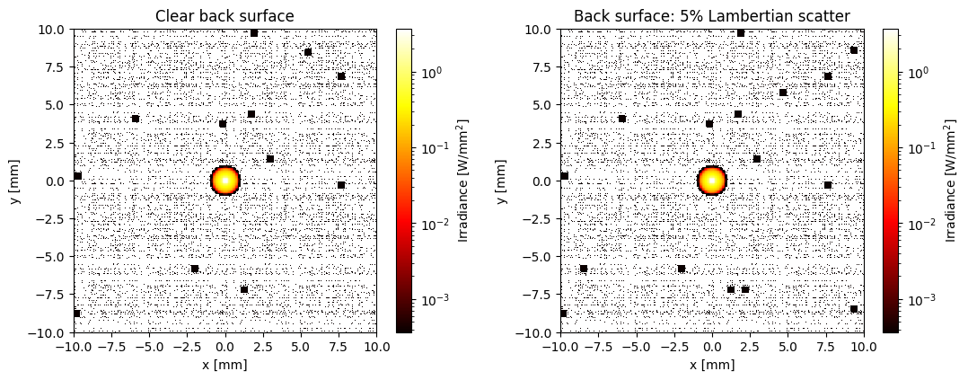
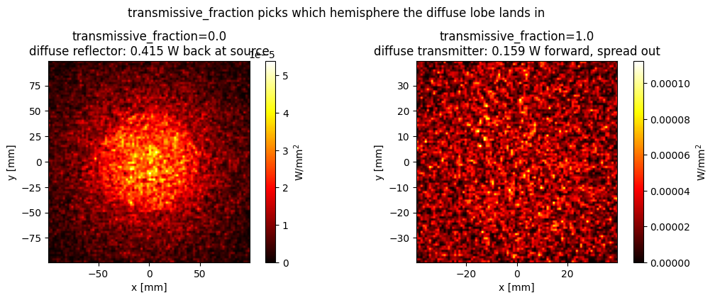
A BSDF replaces the specular or refractive behaviour for the rays it handles, so attaching one with the default settings turns a surface into a pure diffuser. Use SurfaceConfig(bsdf=..., scatter_fraction=f) to send only a fraction f of the light through the scatter model and keep the rest specular, which is how a real partially scattering surface behaves.

Coatings, mirror reflectance & absorption

Reflectance comes from the same optiland.coatings models the sequential engine uses, so the two engines agree on R. Attach one via SurfaceConfig(coating=...) on a lens/doublet face; with no coating, a refractive surface falls back to bare Fresnel. A glass with a nonzero extinction coefficient k attenuates flux automatically via Beer-Lambert absorption over its path length — no extra configuration needed. See notebook 5.

Diagnostics

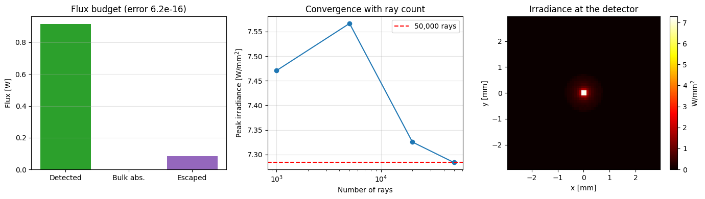
Every trace’s result.diagnostics flags depth-truncated flux, Russian- roulette loss, unreached geometry, and undersampled detectors. Call print(result.report()) after every trace — it is the fastest way to catch a misconfigured scene before trusting its numbers. See notebook 6.

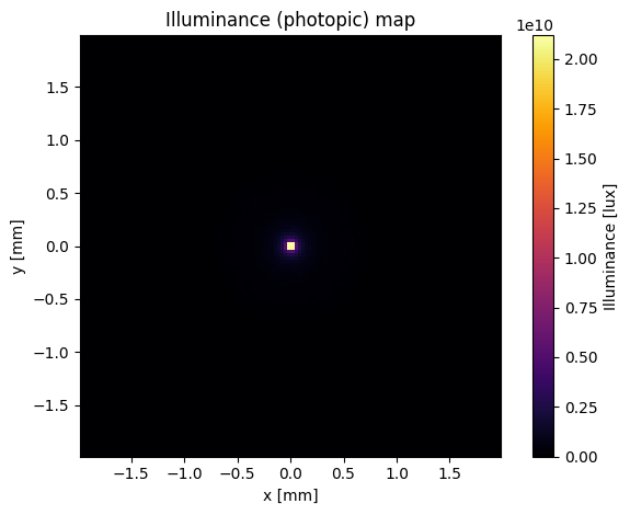
Photometric units

The trace loop is radiometric (watts) throughout; optiland.nonsequential.units.to_photometric() converts a traced detector result to lux/lumens for illumination-engineering workflows, and sources accept total_flux_lumens directly.

Sequential conversion

sequential_to_nonsequential(optic) converts an existing sequential Optic design to an NSQScene automatically, mapping singlets → Lens, cemented doublets → Doublet, and the image surface → IrradianceDetector. Coatings and mirror reflectance are carried over where possible; scene.conversion_report lists exactly what was carried over, defaulted, estimated, or dropped.

Quick-start example

from optiland.coordinate_system import CoordinateSystem
from optiland.nonsequential import (
    NSQScene, Spectrum,
    PointSourceConfig, LensConfig, IrradianceDetectorConfig,
)

scene = NSQScene()
spec = Spectrum.monochromatic(0.55)   # 550 nm

scene.add_source('S', CoordinateSystem(z=-100),
                 PointSourceConfig(spectrum=spec, total_flux=1.0, half_angle_deg=15))
scene.add_lens('L', CoordinateSystem(z=0),
               LensConfig(r1=50, r2=-50, thickness=5, material='N-BK7',
                           front_aperture_radius=12.5))
scene.add_detector('D', CoordinateSystem(z=110),
                   IrradianceDetectorConfig(width=20, height=20))

result = scene.trace(num_rays=100_000, seed=42)
print(result.report())      # catch a misconfigured scene before trusting it
result.detectors['D'].plot()

This quickstart runs on the NumPy forward engine. To get gradients, call be.set_backend("torch") before building the scene and optimize scene parameters with loss.backward() — see notebook 11.

Examples#

Getting Started with Non-Sequential Ray Tracing

Ray Sources

Optical Components

Detectors and Results

Surface Scattering and BSDF Models

Simulation Diagnostics

Multi-Source Illumination

Stray Light Analysis

Reflective and Catadioptric Systems

Advanced Topics

Differentiable Illumination Optimization