Optical Components

The NSQ engine provides three built-in compound components — high-level objects that assemble multiple physical surfaces automatically:

Class	Surfaces created	Typical use
Lens	Front face, back face, edge, optional rim	Single refractive element
Doublet	Front, cemented interface, back, edge	Cemented achromatic doublet
Mirror	One reflective conic surface	Parabolic/spherical mirror

Each compound component is created with a config dataclass that contains all geometric and material parameters. This notebook shows how to configure each type, use the Optiland glass catalog, and apply per-surface overrides.

import matplotlib.pyplot as plt
import numpy as np
from matplotlib.colors import LogNorm

from optiland.coordinate_system import CoordinateSystem
from optiland.coatings import SimpleCoating
from optiland.nonsequential import (
    NSQScene, Spectrum,
    CollimatedSourceConfig,
    IrradianceDetectorConfig,
    LensConfig, DoubletConfig, MirrorConfig,
    SurfaceConfig, InteractionType,
    NSQMaterial, VACUUM,
    LambertianBSDF,
)

spec = Spectrum.monochromatic(0.55)  # 550 nm

1. Materials

LensConfig.material accepts either a glass catalog name string or an NSQMaterial instance.

Using the glass catalog:

# Look up glass by catalog name - same names as the sequential engine
nbk7 = NSQMaterial.from_glass('N-BK7')
nsf11 = NSQMaterial.from_glass('N-SF11')

wl = np.array([0.45, 0.55, 0.65])
print("N-BK7  refractive index at 450/550/650 nm:", nbk7.n(wl).round(5))
print("N-SF11 refractive index at 450/550/650 nm:", nsf11.n(wl).round(5))

# VACUUM is a built-in constant: n = 1.0 everywhere
print("VACUUM refractive index at 550 nm       :", VACUUM.n(0.55))

N-BK7  refractive index at 450/550/650 nm: [1.52532 1.51852 1.51452]
N-SF11 refractive index at 450/550/650 nm: [1.81916 1.79115 1.77663]
VACUUM refractive index at 550 nm       : 1.0

2. Lens

LensConfig defines a singlet. Required fields:

• r1, r2 — radii of curvature [mm] (positive = centre on +z side)

• thickness — centre thickness [mm]

• material — glass name or NSQMaterial

• front_aperture_radius — semi-diameter [mm]

Optional: conic1, conic2 for aspheric surfaces (0 = sphere).

The lens automatically creates an absorbing cylindrical edge and, when front and back apertures differ, an annular rim plane.

def trace_through_lens(lens_config, source_z=-80, detector_z=52.5, n_rays=30_000):
    scene = NSQScene()
    scene.add_source(
        'S', CoordinateSystem(z=source_z),
        CollimatedSourceConfig(spectrum=spec, total_flux=1.0, aperture_radius=10.0),
    )
    scene.add_lens('L', CoordinateSystem(z=0), lens_config)
    scene.add_detector(
        'D', CoordinateSystem(z=detector_z),
        IrradianceDetectorConfig(width=6, height=6, num_pixels_x=128, num_pixels_y=128),
    )
    result = scene.trace(num_rays=n_rays, seed=42)
    # A separate, tiny trace for the picture: recording ray paths runs a
    # Python loop per event, so it belongs nowhere near the statistical trace.
    scene.view(num_rays=60, color_by='bounce')
    plt.show()
    return result.detectors['D']

# Biconvex N-FK5 lens
biconvex = LensConfig(r1=50, r2=-50, thickness=5, material='N-FK5',
                      front_aperture_radius=12.5)

# Plano-convex N-LASF9 lens
planoconvex = LensConfig(r1=40, r2=np.inf, thickness=5, material='N-LASF9',
                         front_aperture_radius=12.5)

# Each lens gets its own detector plane. N-FK5 and N-LASF9 have different
# indices, so two lenses with the same radii do not share a focus, and a
# plano-convex has a different back focal distance again.
irr_biconvex    = trace_through_lens(biconvex,    detector_z=52.5)
irr_planoconvex = trace_through_lens(planoconvex, detector_z=49.0)

fig, axes = plt.subplots(1, 2, figsize=(10, 4))
for ax, irr, title in zip(axes, [irr_biconvex, irr_planoconvex],
                          ['Biconvex N-FK5 (focus z = 52.5)',
                           'Plano-convex N-LASF9 (focus z = 49.0)']):
    im = ax.imshow(irr.irradiance, origin='lower', cmap='hot', aspect='equal',
                   extent=[irr.x_coords[0], irr.x_coords[-1],
                            irr.y_coords[0], irr.y_coords[-1]])
    plt.colorbar(im, ax=ax, label='W/mm²')
    ax.set_title(title)
    ax.set_xlabel('x [mm]'); ax.set_ylabel('y [mm]')
plt.tight_layout()
plt.show()

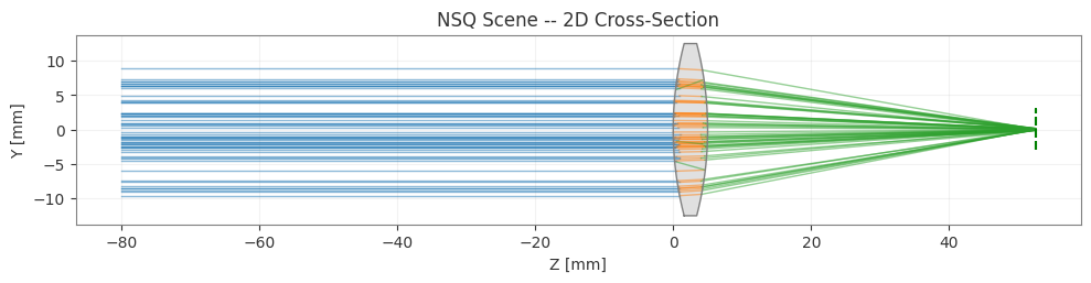
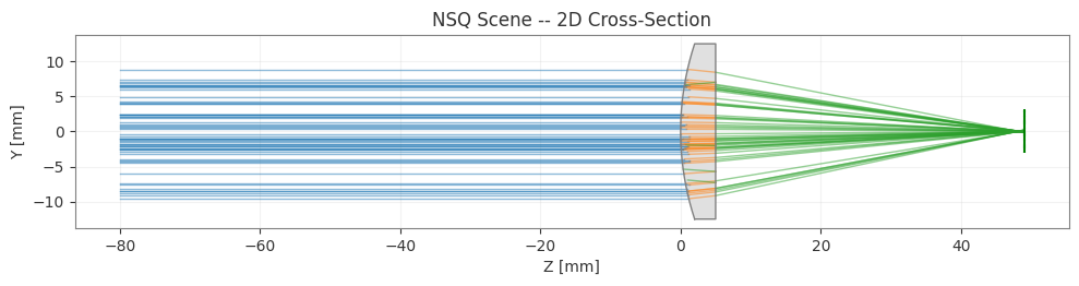
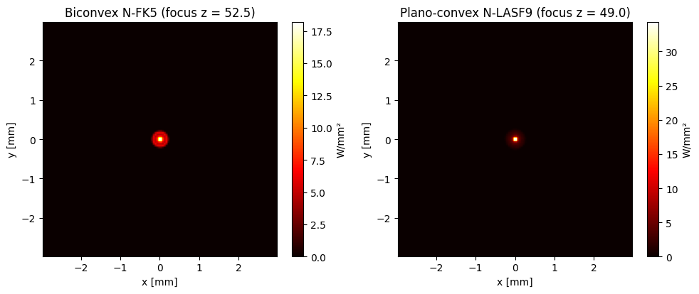
3. Doublet (Cemented Achromat)

A Doublet consists of a crown element (material1) and a flint element (material2) cemented together. It has three radii of curvature and two thicknesses.

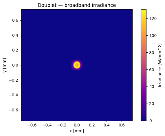
Using a broadband spectrum reveals the chromatic correction:

spec_rgb = Spectrum(
    wavelengths=np.array([0.45, 0.55, 0.65]),
    weights=np.array([1.0, 1.0, 1.0]),
)

doublet_config = DoubletConfig(
    r1=60.0, r2=-60.0, r3=-300.0,
    thickness1=5.0, thickness2=3.0,
    material1='N-BK7', material2='N-SF5',
    aperture_radius=12.5,
)

scene = NSQScene()
scene.add_source(
    'S', CoordinateSystem(z=-80),
    CollimatedSourceConfig(spectrum=spec_rgb, total_flux=1.0, aperture_radius=10.0),
)
scene.add_doublet('D1', CoordinateSystem(z=0), doublet_config)
# This doublet focuses at z = 124 mm, found by scanning the spot size along
# the axis. Guessing the plane is the fastest way to mistake defocus for
# aberration.
scene.add_detector(
    'Det', CoordinateSystem(z=124),
    IrradianceDetectorConfig(width=1.5, height=1.5, num_pixels_x=128, num_pixels_y=128),
)

scene.view(num_rays=60, color_by='bounce')
plt.show()

result = scene.trace(num_rays=30_000, seed=42)
irr = result.detectors['Det']

print(f"Doublet surfaces   : {len(scene.surfaces)}")
print(f"Rays on detector   : {irr.num_rays_hit:,}")
print(f"Flux on detector   : {irr.total_flux:.4f} W")

fig = irr.plot(cmap='plasma')
plt.title('Doublet — broadband irradiance')
plt.tight_layout()
plt.show()

Doublet surfaces   : 5
Rays on detector   : 26,873
Flux on detector   : 0.8918 W

4. Mirror

MirrorConfig has four parameters:

• radius — vertex radius of curvature [mm]. Negative = concave when facing +z

• reflectance — required, no default. A constant in [0, 1], a callable(wavelength_um) -> reflectance, or an unpolarized optiland.coatings coating.

• conic — conic constant (0 = sphere, -1 = paraboloid, <−1 = hyperboloid)

• aperture_radius — semi-diameter [mm]

reflectance has no implicit default because a mirror built without specifying how much light it reflects is a modelling bug, not a real 100%-reflecting surface: MirrorConfig(radius=-200, conic=-1.0, aperture_radius=25.0) (no reflectance) raises TypeError rather than silently giving you a perfect mirror. Below we use reflectance=0.95, typical of a protected-aluminum first-surface mirror; reflectance can also be a callable of wavelength for a dichroic or metal coating with real dispersion, or an optiland.coatings object.

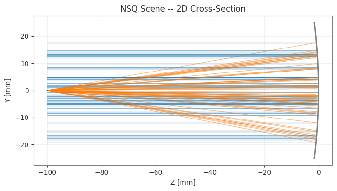
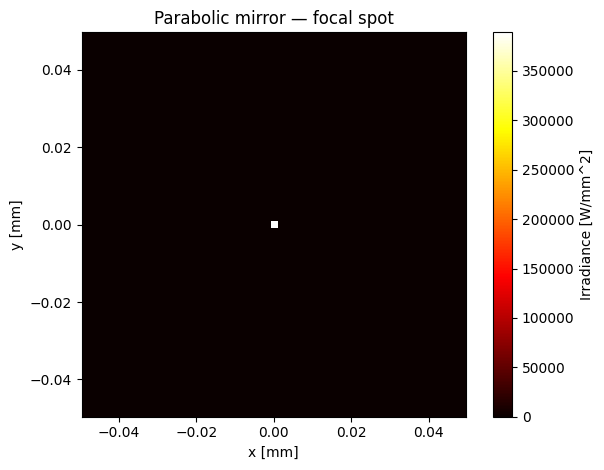
A parabolic mirror (conic=-1) focuses a collimated on-axis beam to a perfect geometrical point (no spherical aberration).

# Parabolic mirror: f = |R|/2 = 100 mm, R = -200 mm.
# reflectance=0.95 models a realistic protected-aluminum coating rather than
# an idealized perfect reflector -- 5% of the incident flux is lost at the
# mirror surface, which shows up directly in the flux budget below.
mirror_config = MirrorConfig(radius=-200, conic=-1.0, aperture_radius=25.0,
                             reflectance=0.95)

scene_m = NSQScene()
scene_m.add_source(
    'S', CoordinateSystem(z=-100),
    CollimatedSourceConfig(spectrum=spec, total_flux=1.0, aperture_radius=20.0),
)
scene_m.add_mirror('M', CoordinateSystem(z=0), mirror_config)

# Focal plane: f = |R|/2 = 100 mm. Mirror is at z=0, beam enters from z<0,
# so the reflected focus is at z = -100 mm.
scene_m.add_detector(
    'Det', CoordinateSystem(z=-100),
    IrradianceDetectorConfig(width=0.1, height=0.1, num_pixels_x=128, num_pixels_y=128),
)

scene_m.view(num_rays=60, color_by='bounce')
plt.show()

result_m = scene_m.trace(num_rays=30_000, seed=42)
irr_m = result_m.detectors['Det']

fig = irr_m.plot(cmap='hot')
plt.title('Parabolic mirror — focal spot')
plt.tight_layout()
plt.show()

print(f"Rays on detector: {irr_m.num_rays_hit:,} | Flux: {irr_m.total_flux:.4f} W")
print(f"(Flux is capped near 0.95 W of the 1.0 W launched -- the 5% the "
      f"mirror does not reflect.)")

Rays on detector: 30,000 | Flux: 0.9500 W
(Flux is capped near 0.95 W of the 1.0 W launched -- the 5% the mirror does not reflect.)

5. AR Coatings

A bare refractive surface reflects a small fraction of the incident light at each interface (bare Fresnel reflectance), which is why an uncoated lens never transmits 100% of the flux that enters it. SurfaceConfig(coating=...) attaches an optiland.coatings model to a LensConfig/DoubletConfig face (via front=/back=) or directly to a RefractiveComponent; its reflectance/transmittance then replace the bare Fresnel calculation, so NSQ and the sequential engine agree on R for the same coating.

SimpleCoating(transmittance, reflectance) is the unpolarized coating model — pass it a small reflectance (e.g. 0.005, i.e. 0.5% per surface, typical of a broadband AR coating) to see the effect. Coatings on refractive surfaces are optional: with none attached, a surface just falls back to bare Fresnel, as in every lens above.

# Same biconvex N-FK5 lens as above, once bare and once with a broadband AR
# coating (0.5% reflectance per surface) on both faces.
ar = SurfaceConfig(coating=SimpleCoating(transmittance=0.995, reflectance=0.005))

biconvex_bare = LensConfig(r1=50, r2=-50, thickness=5, material='N-FK5',
                           front_aperture_radius=12.5)
biconvex_coated = LensConfig(r1=50, r2=-50, thickness=5, material='N-FK5',
                             front_aperture_radius=12.5, front=ar, back=ar)


def flux_through(lens_config, detector_z=52.5, n_rays=100_000):
    scene = NSQScene()
    scene.add_source(
        'S', CoordinateSystem(z=-80),
        CollimatedSourceConfig(spectrum=spec, total_flux=1.0, aperture_radius=10.0),
    )
    scene.add_lens('L', CoordinateSystem(z=0), lens_config)
    scene.add_detector(
        'D', CoordinateSystem(z=detector_z),
        IrradianceDetectorConfig(width=6, height=6, num_pixels_x=128, num_pixels_y=128),
    )
    return scene.trace(num_rays=n_rays, seed=42).detectors['D']


irr_bare = flux_through(biconvex_bare)
irr_coated = flux_through(biconvex_coated)

print(f"Bare (Fresnel) lens : {irr_bare.total_flux:.4f} W on detector")
print(f"AR-coated lens      : {irr_coated.total_flux:.4f} W on detector")
print(f"Extra throughput from coating: "
      f"{100 * (irr_coated.total_flux / irr_bare.total_flux - 1):.2f}%")
print()
print("Two surfaces each reflecting a few percent by bare Fresnel add up: the")
print("AR coating recovers that loss and delivers more flux to the same spot.")

Bare (Fresnel) lens : 0.9232 W on detector
AR-coated lens      : 0.9884 W on detector
Extra throughput from coating: 7.06%

Two surfaces each reflecting a few percent by bare Fresnel add up: the
AR coating recovers that loss and delivers more flux to the same spot.

6. Per-Surface Overrides with SurfaceConfig

LensConfig.front, .back, .edge, and .rim accept a SurfaceConfig to override defaults on a per-surface basis:

• interaction — force REFRACTIVE, REFLECTIVE, or ABSORBING

• bsdf — attach a scatter model (see the Scattering notebook)

• scatter_fraction — how much of the light the BSDF handles

• aperture_radius — override the semi-diameter for that surface

• coating — attach an AR/reflective coating (see above)

How a BSDF interacts with the surface

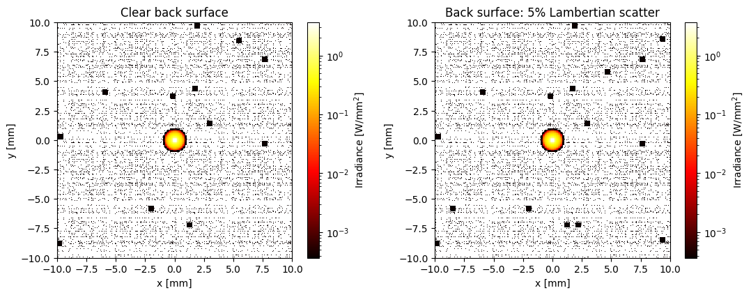
A BSDF replaces the surface’s specular behaviour for the rays it handles: a ray routed to a LambertianBSDF is scattered into the diffuse hemisphere instead of being refracted. scatter_fraction sets how many rays that is.

• scatter_fraction=1.0 (the default) makes the surface a pure diffuser — no light continues along the refracted path.

• scatter_fraction=0.05 makes it mostly clear with a slight haze, which is what a real scratched or lightly frosted surface looks like.

Below the back face of the lens scatters 5% of the light diffusely and refracts the other 95% normally, so the focused spot and the diffuse veil appear together.

# Lens whose back face scatters 5% of the light into a Lambertian hemisphere
# and refracts the remaining 95% as usual.
scatter_config = LensConfig(
    r1=50, r2=-50, thickness=5, material='N-BK7',
    front_aperture_radius=12.5,
    back=SurfaceConfig(
        bsdf=LambertianBSDF(reflectance_value=0.9),  # 90% of scattered flux survives
        scatter_fraction=0.05,                       # 5% of rays are scattered
    ),
)

scene_sc = NSQScene()
scene_sc.add_source(
    'S', CoordinateSystem(z=-80),
    CollimatedSourceConfig(spectrum=spec, total_flux=1.0, aperture_radius=10.0),
)
scene_sc.add_lens('L', CoordinateSystem(z=0), scatter_config)
scene_sc.add_detector(
    'D', CoordinateSystem(z=52.4),
    IrradianceDetectorConfig(width=20, height=20, num_pixels_x=128, num_pixels_y=128),
)

result_sc = scene_sc.trace(num_rays=100_000, seed=42)
irr_sc = result_sc.detectors['D']

# Compare against the same lens with no scatter at all.
clear_config = LensConfig(r1=50, r2=-50, thickness=5, material='N-BK7',
                          front_aperture_radius=12.5)
scene_clear = NSQScene()
scene_clear.add_source(
    'S', CoordinateSystem(z=-80),
    CollimatedSourceConfig(spectrum=spec, total_flux=1.0, aperture_radius=10.0),
)
scene_clear.add_lens('L', CoordinateSystem(z=0), clear_config)
scene_clear.add_detector(
    'D', CoordinateSystem(z=52.4),
    IrradianceDetectorConfig(width=20, height=20, num_pixels_x=128, num_pixels_y=128),
)
irr_clear = scene_clear.trace(num_rays=100_000, seed=42).detectors['D']

print(f"Clear lens      : {irr_clear.total_flux:.4f} W on detector")
print(f"5% diffuse back : {irr_sc.total_flux:.4f} W on detector")

# A log scale shows the faint diffuse veil next to the bright core.
fig, axes = plt.subplots(1, 2, figsize=(11, 4.2))
extent = [-10, 10, -10, 10]
vmax = max(irr_clear.irradiance.max(), irr_sc.irradiance.max())
for ax, irr, title in zip(
    axes,
    [irr_clear.irradiance, irr_sc.irradiance],
    ['Clear back surface', 'Back surface: 5% Lambertian scatter'],
):
    im = ax.imshow(irr, origin='lower', extent=extent, cmap='hot',
                   norm=LogNorm(vmin=vmax * 1e-4, vmax=vmax))
    ax.set_title(title)
    ax.set_xlabel('x [mm]')
    ax.set_ylabel('y [mm]')
    plt.colorbar(im, ax=ax, label='Irradiance [W/mm$^2$]')

plt.tight_layout()
plt.show()

Clear lens      : 0.9166 W on detector
5% diffuse back : 0.8716 W on detector

Summary

• LensConfig(r1, r2, thickness, material, front_aperture_radius) — singlet refractive element

• DoubletConfig(r1, r2, r3, thickness1, thickness2, material1, material2, aperture_radius) — cemented achromat

• MirrorConfig(radius, reflectance, conic, aperture_radius) — conic reflective mirror; reflectance is required (constant, callable, or coating) — there is no implicit 100%-reflecting default

• Glass names ('N-BK7', 'N-SF5', …) are looked up in the Optiland material catalog

• SurfaceConfig(coating=...) attaches an optiland.coatings model (e.g. SimpleCoating) to a refractive face, replacing bare Fresnel reflectance — the same coating model the sequential engine uses

• SurfaceConfig overrides individual surface properties (BSDF, interaction type, aperture, coating)

• SurfaceConfig(bsdf=..., scatter_fraction=f) makes a surface partially scattering: a fraction f of rays go to the BSDF, the rest keep the specular/refractive path

• VACUUM constant for a lossless n=1 medium