Surface Scattering and BSDF Models

A BSDF (Bidirectional Scattering Distribution Function) describes how a surface redirects light that is not simply refracted or specularly reflected.

BSDF	Scatter type	Parameters
Default (None)	Specular Fresnel refraction/reflection	–
SpecularBRDF	Perfect mirror reflection	–
LambertianBSDF	Cosine-weighted diffuse scatter	reflectance_value in [0,1]
HarveyShackBSDF	Micro-roughness scatter (ABg model)	b0, l0, s
TabulatedBSDF	User-defined lookup table	angles + BRDF values

Attach one through a SurfaceConfig:

SurfaceConfig(bsdf=LambertianBSDF(0.9), scatter_fraction=0.05)

Two separate ideas are at work here, and keeping them apart avoids most of the confusion around scatter models:

• The BSDF sets the shape of the scatter lobe – where a scattered ray goes.

• ``scatter_fraction`` sets how much light is scattered – the probability that a ray striking the surface is handed to the BSDF at all. The rest continue along the ordinary specular or refractive path.

A BSDF replaces the specular behaviour for the rays it handles, so scatter_fraction=1.0 (the default) turns a surface into a pure diffuser with no transmitted beam left. Real surfaces scatter a small fraction, so a value well below 1 is usually what you want.

import matplotlib.pyplot as plt
import numpy as np
from matplotlib.colors import LogNorm

from optiland.coordinate_system import CoordinateSystem
from optiland.nonsequential import (
    NSQScene, Spectrum,
    CollimatedSourceConfig, PointSourceConfig,
    IrradianceDetectorConfig,
    LensConfig, MirrorConfig,
    SurfaceConfig,
    SpecularBRDF, LambertianBSDF, HarveyShackBSDF,
)

spec = Spectrum.monochromatic(0.55)

1. Default Behaviour: Fresnel Refraction

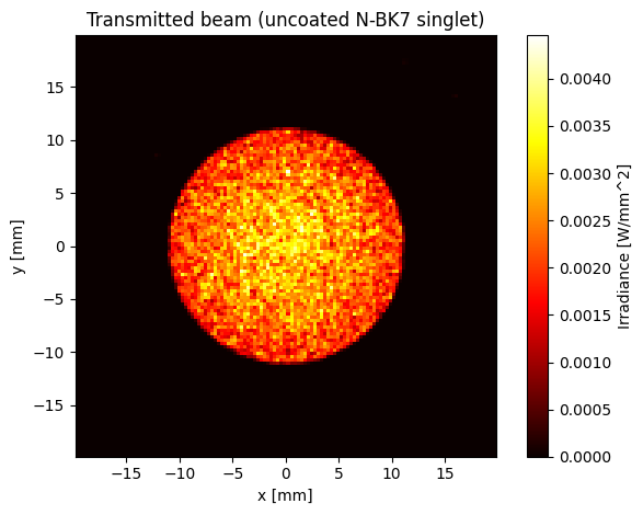
With no BSDF, a refractive surface uses detached-sample / attached-weight Fresnel splitting: each ray is stochastically either refracted or reflected according to the Fresnel equations, with a throughput weight that keeps the estimate unbiased (and differentiable on the torch backend). This is the physically correct treatment for uncoated glass.

At normal incidence N-BK7 reflects about 4% per surface, so a lens with two uncoated faces transmits roughly 92%.

Note the detector is deliberately made large enough to catch the entire diverging beam. Sizing it too small removes flux that was transmitted perfectly well, and the missing light then looks like a surface loss.

scene = NSQScene()
scene.add_source(
    'S', CoordinateSystem(z=-80),
    CollimatedSourceConfig(spectrum=spec, total_flux=1.0, aperture_radius=10.0),
)
scene.add_lens(
    'L', CoordinateSystem(z=0),
    LensConfig(r1=50, r2=-50, thickness=5, material='N-BK7', front_aperture_radius=12.5),
)
# 40 mm across: past focus the beam has spread to ~21 mm diameter, so a
# 20 mm detector would clip it and understate the transmission.
scene.add_detector(
    'D', CoordinateSystem(z=100),
    IrradianceDetectorConfig(width=40, height=40, num_pixels_x=128, num_pixels_y=128),
)

result = scene.trace(num_rays=50_000, seed=42)
irr = result.detectors['D']

transmission = irr.total_flux / result.total_flux_in * 100
print(f"Flux in       : {result.total_flux_in:.4f} W")
print(f"Flux detected : {irr.total_flux:.4f} W")
print(f"Transmission  : {transmission:.1f}%")
print(f"Fresnel loss  : {100 - transmission:.1f}%  (expected ~8% for two uncoated surfaces)")

fig = irr.plot(cmap='hot')
plt.title('Transmitted beam (uncoated N-BK7 singlet)')
plt.tight_layout()
plt.show()

Flux in       : 1.0000 W
Flux detected : 0.9166 W
Transmission  : 91.7%
Fresnel loss  : 8.3%  (expected ~8% for two uncoated surfaces)

2. SpecularBRDF: Perfect Mirror

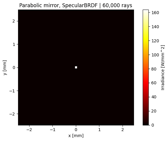
SpecularBRDF reflects every ray about the surface normal with no loss and no spread. It is useful for an idealised mirror.

The mirror below is concave toward the incoming beam, which is expressed by a negative radius (centre of curvature on the -z side). No rotation is needed; adding one would flip it to convex and diverge the beam.

MirrorConfig.reflectance has no implicit default and is a required argument – a mirror built without one raises, so a scene never silently gets a 100% reflector. Here it is set to 1.0 deliberately, since the point of this section is to isolate the directional behaviour of SpecularBRDF from any flux loss; a real mirror coating would use a lower value (see the MirrorConfig docstring for constants, wavelength-dependent callables, or optiland.coatings objects).

# Parabolic mirror, f = |radius| / 2 = 100 mm
scene_spec = NSQScene()
scene_spec.add_source(
    'S', CoordinateSystem(z=-80),
    CollimatedSourceConfig(spectrum=spec, total_flux=1.0, aperture_radius=15.0),
)
scene_spec.add_mirror(
    'M', CoordinateSystem(z=0),
    MirrorConfig(radius=-200, conic=-1.0, aperture_radius=20.0, reflectance=1.0,
                 surface=SurfaceConfig(bsdf=SpecularBRDF())),
)
scene_spec.add_detector(
    'D', CoordinateSystem(z=-100),   # at the focus
    IrradianceDetectorConfig(width=5, height=5, num_pixels_x=128, num_pixels_y=128),
)

result_spec = scene_spec.trace(num_rays=60_000, seed=42)
irr_spec = result_spec.detectors['D']

print(f"Flux on detector: {irr_spec.total_flux:.4f} W of {result_spec.total_flux_in:.1f} W")

fig = irr_spec.plot(cmap='hot')
plt.title(f'Parabolic mirror, SpecularBRDF | {irr_spec.num_rays_hit:,} rays')
plt.tight_layout()
plt.show()

Flux on detector: 1.0000 W of 1.0 W

3. LambertianBSDF: Diffuse Scatter

LambertianBSDF(reflectance_value) scatters rays into a cosine-weighted hemisphere about the surface normal, the standard model for a matte surface. reflectance_value scales the flux of each scattered ray, so 0.9 means 10% is absorbed at the scatter event.

Because the scatter is built about the normal facing the incoming ray, a diffuse surface sends light back toward the source: it is a diffuse reflector, not a diffuser you can see through.

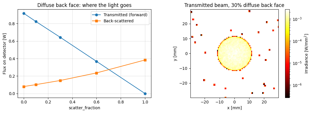
scatter_fraction decides how much of the beam is treated this way. Below, the back face of a lens scatters a varying fraction and refracts the rest, so the transmitted beam and the back-scattered light trade off against each other.

lambertian = LambertianBSDF(reflectance_value=0.9)


def trace_scatter(fraction, n_rays=40_000):
    """Lens whose back face scatters `fraction` of the light diffusely."""
    scene_l = NSQScene()
    scene_l.add_source(
        'S', CoordinateSystem(z=-80),
        CollimatedSourceConfig(spectrum=spec, total_flux=1.0, aperture_radius=10.0),
    )
    scene_l.add_lens(
        'L', CoordinateSystem(z=0),
        LensConfig(
            r1=50, r2=-50, thickness=5, material='N-BK7',
            front_aperture_radius=12.5,
            back=SurfaceConfig(bsdf=lambertian, scatter_fraction=fraction),
        ),
    )
    # Forward detector past the focus, backward detector behind the source
    scene_l.add_detector(
        'D_fwd', CoordinateSystem(z=100),
        IrradianceDetectorConfig(width=60, height=60, num_pixels_x=96, num_pixels_y=96),
    )
    scene_l.add_detector(
        'D_bwd', CoordinateSystem(z=-90),
        IrradianceDetectorConfig(width=200, height=200, num_pixels_x=96, num_pixels_y=96),
    )
    res = scene_l.trace(num_rays=n_rays, seed=42)
    return res.detectors['D_fwd'], res.detectors['D_bwd']


fractions = [0.0, 0.1, 0.3, 0.6, 1.0]
fwd_flux, bwd_flux = [], []
for f in fractions:
    fwd, bwd = trace_scatter(f)
    fwd_flux.append(fwd.total_flux)
    bwd_flux.append(bwd.total_flux)
    print(f"scatter_fraction={f:4.1f} -> forward {fwd.total_flux:.3f} W, "
          f"back-scattered {bwd.total_flux:.3f} W")

fig, axes = plt.subplots(1, 2, figsize=(11, 4))

ax = axes[0]
ax.plot(fractions, fwd_flux, 'o-', label='Transmitted (forward)')
ax.plot(fractions, bwd_flux, 's-', label='Back-scattered')
ax.set_xlabel('scatter_fraction')
ax.set_ylabel('Flux on detector [W]')
ax.set_title('Diffuse back face: where the light goes')
ax.legend()
ax.grid(True, alpha=0.4)

# Spatial picture at a 30% scatter fraction
fwd30, _ = trace_scatter(0.3)
ax = axes[1]
im = ax.imshow(fwd30.irradiance, origin='lower', cmap='hot',
               extent=[fwd30.x_coords[0], fwd30.x_coords[-1],
                       fwd30.y_coords[0], fwd30.y_coords[-1]],
               norm=LogNorm(vmin=fwd30.irradiance.max() * 1e-4,
                            vmax=fwd30.irradiance.max()))
plt.colorbar(im, ax=ax, label='Irradiance [W/mm$^2$]')
ax.set_title('Transmitted beam, 30% diffuse back face')
ax.set_xlabel('x [mm]')
ax.set_ylabel('y [mm]')

plt.tight_layout()
plt.show()

scatter_fraction= 0.0 -> forward 0.916 W, back-scattered 0.080 W
scatter_fraction= 0.1 -> forward 0.823 W, back-scattered 0.102 W
scatter_fraction= 0.3 -> forward 0.643 W, back-scattered 0.149 W
scatter_fraction= 0.6 -> forward 0.368 W, back-scattered 0.236 W
scatter_fraction= 1.0 -> forward 0.000 W, back-scattered 0.384 W

4. HarveyShackBSDF: Micro-Roughness Scatter

The Harvey-Shack ABg model describes scatter from a polished surface’s residual micro-roughness. It is written in direction-cosine space:

\[\mathrm{BSDF}\left(|\beta - \beta_0|\right) = \frac{b_0}{1 + \left(|\beta - \beta_0| / l_0\right)^{s}}\]

where \(\beta_0\) is the specular direction and \(\beta\) the scattered one.

• b0 sets the scatter level at the specular peak

• l0 is the break frequency, i.e. the angular width of the lobe

• s is the roll-off exponent: larger means the tail falls away faster

Two separate quantities follow from these parameters:

• The lobe shape, which the BSDF samples directly.

• The total integrated scatter (TIS), available as bsdf.total_integrated_scatter. This is the fraction of incident power a real surface with these parameters would scatter, and is the natural value for scatter_fraction.

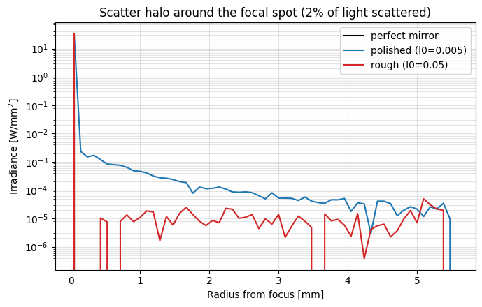
A polished mirror has a TIS of order \(10^{-5}\), so essentially all light stays specular and the scatter forms a faint halo around a bright core, exactly the veiling glare that limits contrast in real instruments.

polished = HarveyShackBSDF(b0=1e-2, l0=0.005, s=2.0)   # tight lobe
rough    = HarveyShackBSDF(b0=1e-2, l0=0.05,  s=1.5)   # broad lobe

for name, bsdf in [('polished', polished), ('rough', rough)]:
    print(f"{name:9s}: l0={bsdf.l0:<6} TIS={bsdf.total_integrated_scatter:.2e}")


def mirror_with_scatter(bsdf, fraction, n_rays=200_000):
    """Parabolic mirror whose surface scatters `fraction` of the light."""
    scene_m = NSQScene()
    scene_m.add_source(
        'S', CoordinateSystem(z=-80),
        CollimatedSourceConfig(spectrum=spec, total_flux=1.0, aperture_radius=15.0),
    )
    scene_m.add_mirror(
        'M', CoordinateSystem(z=0),
        MirrorConfig(radius=-200, conic=-1.0, aperture_radius=20.0, reflectance=1.0,
                     surface=SurfaceConfig(bsdf=bsdf, scatter_fraction=fraction)),
    )
    scene_m.add_detector(
        'D', CoordinateSystem(z=-100),
        IrradianceDetectorConfig(width=8, height=8, num_pixels_x=160, num_pixels_y=160),
    )
    return scene_m.trace(num_rays=n_rays, seed=42).detectors['D']


def radial_profile(irr):
    """Azimuthally averaged irradiance versus radius."""
    X, Y = np.meshgrid(irr.x_coords, irr.y_coords)
    R = np.hypot(X, Y).ravel()
    E = irr.irradiance.ravel()
    bins = np.linspace(0, R.max(), 60)
    idx = np.digitize(R, bins) - 1
    prof = np.array([E[idx == k].mean() if np.any(idx == k) else np.nan
                     for k in range(len(bins) - 1)])
    return 0.5 * (bins[:-1] + bins[1:]), prof


# 2% scattered so the halo is visible above Monte Carlo noise; a real polished
# mirror would use scatter_fraction = bsdf.total_integrated_scatter.
fig, ax = plt.subplots(figsize=(7, 4.5))
for label, bsdf, colour in [('perfect mirror', None, 'k'),
                            ('polished (l0=0.005)', polished, 'tab:blue'),
                            ('rough (l0=0.05)', rough, 'tab:red')]:
    irr_m = (mirror_with_scatter(bsdf, 0.02) if bsdf is not None
             else mirror_with_scatter(SpecularBRDF(), 0.0))
    r, prof = radial_profile(irr_m)
    ax.semilogy(r, prof, color=colour, label=label)

ax.set_xlabel('Radius from focus [mm]')
ax.set_ylabel('Irradiance [W/mm$^2$]')
ax.set_title('Scatter halo around the focal spot (2% of light scattered)')
ax.legend()
ax.grid(True, alpha=0.35, which='both')
plt.tight_layout()
plt.show()

polished : l0=0.005  TIS=9.41e-06
rough    : l0=0.05   TIS=1.61e-03

5. Inspecting a BSDF Directly

Every BSDF exposes sample(num_rays, incident_dirs, normals, wavelengths, rng, ray_id, bounce), returning (scattered_dirs, flux_weights, transmitted). Calling it yourself is the clearest way to see what a model does, with no scene geometry in the way.

rng is an NSQRng – the engine’s keyed PCG32 (see the developer guide’s Reproducibility section), not a plain numpy.random.Generator: every draw is a pure function of (seed, ray_id, bounce, event_slot), so ray_id and bounce must be supplied per sample. Below, each of the N_SAMPLES calls gets its own ray_id (bounce=0 throughout) so every draw is independent.

Below, a beam travelling along \(+z\) strikes a surface whose normal faces \(-z\), so the specular direction is \(-z\) and the polar angle \(\theta\) is measured from it.

For a Lambertian surface the density of scattered rays over \(\theta\) is

\[p(\theta) = \sin(2\theta), \qquad \langle\cos\theta\rangle = \tfrac{2}{3}\]

which peaks at 45 degrees. This is the signature of cosine weighting: a uniform hemisphere would instead give \(p(\theta) = \sin\theta\) and \(\langle\cos\theta\rangle = 1/2\).

from optiland.nonsequential import NSQRng

rng = NSQRng(seed=0)
N_SAMPLES = 200_000

# Beam along +z hitting a surface whose normal faces -z: specular is -z.
incident = np.tile([0.0, 0.0, 1.0], (N_SAMPLES, 1))
normals = np.tile([0.0, 0.0, -1.0], (N_SAMPLES, 1))
wavelengths = np.full(N_SAMPLES, 0.55)
# A distinct ray_id per sample (bounce=0 throughout) is what makes every draw
# independent under NSQRng's keyed PCG32.
ray_id = np.arange(N_SAMPLES)
bounce = np.zeros(N_SAMPLES, dtype=np.int64)

fig, axes = plt.subplots(1, 2, figsize=(12, 4.2))

# ---- Lambertian: cosine-weighted, peaking at 45 degrees --------------------
dirs_lam, _, _ = LambertianBSDF(1.0).sample(
    N_SAMPLES, incident, normals, wavelengths, rng, ray_id, bounce
)
theta_lam = np.degrees(np.arccos(np.clip(-np.asarray(dirs_lam)[:, 2], -1.0, 1.0)))

ax = axes[0]
ax.hist(theta_lam, bins=60, range=(0, 90), density=True,
        alpha=0.65, label='Sampled')
theta_ref = np.linspace(0, 90, 200)
# sin(2*theta) expressed as a density per degree
ax.plot(theta_ref, np.sin(2 * np.radians(theta_ref)) * np.pi / 180,
        'r--', lw=2, label=r'Theory  $\sin(2\theta)$')
ax.set_xlabel(r'$\theta$ from surface normal [deg]')
ax.set_ylabel('Probability density [1/deg]')
ax.set_title('LambertianBSDF: cosine-weighted hemisphere')
ax.legend()
ax.grid(True, alpha=0.35)

# ---- Harvey-Shack: narrow lobe about the specular direction ----------------
ax = axes[1]
for label, bsdf, colour in [('polished (l0=0.005)', polished, 'tab:blue'),
                            ('rough (l0=0.05)', rough, 'tab:red')]:
    dirs_hs, _, _ = bsdf.sample(N_SAMPLES, incident, normals, wavelengths, rng, ray_id, bounce)
    theta_hs = np.degrees(np.arccos(np.clip(-np.asarray(dirs_hs)[:, 2], -1.0, 1.0)))
    ax.hist(theta_hs, bins=np.logspace(-2, 2, 60), density=True,
            histtype='step', lw=2, color=colour, label=label)

ax.set_xscale('log')
ax.set_yscale('log')
ax.set_xlabel(r'$\theta$ from specular [deg]')
ax.set_ylabel('Probability density [1/deg]')
ax.set_title('HarveyShackBSDF: ABg lobe about specular')
ax.legend()
ax.grid(True, alpha=0.35, which='both')

plt.tight_layout()
plt.show()

print(f"Lambertian <cos(theta)> = {np.mean(np.cos(np.radians(theta_lam))):.4f} "
      f"(exact 2/3 = {2 / 3:.4f})")

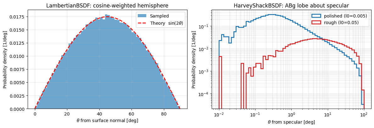
Lambertian <cos(theta)> = 0.6673 (exact 2/3 = 0.6667)

6. Transmissive Lambertian: a Diffuser You Can See Through

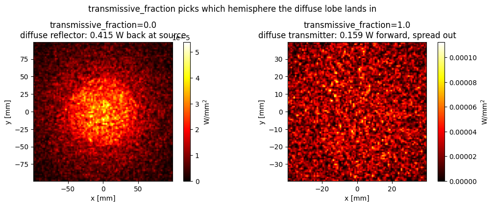
Section 3’s diffuse back face only ever sent light back toward the source, because the scatter lobe was built about the normal facing the incoming ray. LambertianBSDF has a second parameter, transmissive_fraction, that changes this: it is the probability that a given scatter event samples the hemisphere on the far side of the surface (built about -normal) instead of the near side. This is the model for a real diffuser you look through – ground glass, an engineered diffuser, a translucent shade – rather than a diffuse mirror.

• transmissive_fraction=0.0 (the default, used implicitly in section 3): every scatter event lands in the reflective hemisphere.

• transmissive_fraction=1.0: every scatter event lands in the transmissive hemisphere – light passes through the surface, spread into a cosine-weighted cone instead of continuing along the specular refraction direction.

Both extremes below use the same lens back face with scatter_fraction=1.0 (a pure diffuser, no direct beam left) so the only thing that changes is which hemisphere the light ends up in.

def trace_transmissive(transmissive_fraction, n_rays=60_000):
    """Lens whose back face is a pure diffuser, split between the
    reflective and transmissive hemispheres by `transmissive_fraction`."""
    diffuser = LambertianBSDF(reflectance_value=0.95,
                              transmissive_fraction=transmissive_fraction)
    scene_t = NSQScene()
    scene_t.add_source(
        'S', CoordinateSystem(z=-80),
        CollimatedSourceConfig(spectrum=spec, total_flux=1.0, aperture_radius=10.0),
    )
    scene_t.add_lens(
        'L', CoordinateSystem(z=0),
        LensConfig(
            r1=50, r2=-50, thickness=5, material='N-BK7',
            front_aperture_radius=12.5,
            back=SurfaceConfig(bsdf=diffuser, scatter_fraction=1.0),
        ),
    )
    scene_t.add_detector(
        'D_fwd', CoordinateSystem(z=100),
        IrradianceDetectorConfig(width=80, height=80, num_pixels_x=96, num_pixels_y=96),
    )
    scene_t.add_detector(
        'D_bwd', CoordinateSystem(z=-90),
        IrradianceDetectorConfig(width=200, height=200, num_pixels_x=96, num_pixels_y=96),
    )
    res = scene_t.trace(num_rays=n_rays, seed=42)
    return res.detectors['D_fwd'], res.detectors['D_bwd']


fwd_reflect, bwd_reflect = trace_transmissive(0.0)   # diffuse reflector
fwd_transmit, bwd_transmit = trace_transmissive(1.0)  # diffuse transmitter

print(f"transmissive_fraction=0.0 (reflector) : forward {fwd_reflect.total_flux:.3f} W, "
      f"backward {bwd_reflect.total_flux:.3f} W")
print(f"transmissive_fraction=1.0 (transmitter): forward {fwd_transmit.total_flux:.3f} W, "
      f"backward {bwd_transmit.total_flux:.3f} W")
print()
print("Forward is exactly 0 W in the reflector case: scatter_fraction=1.0 means the "
      "back face has no direct specular path left, so nothing reaches D_fwd on axis.")
print("Backward is nonzero (~0.04 W) even in the transmitter case: that is the front "
      "face's own ~4% Fresnel reflection (section 1), unrelated to the back-face BSDF, "
      "so it shows up on D_bwd regardless of transmissive_fraction.")
print("Forward flux in the transmitter case is far below the ~0.87 W actually leaving "
      "the back face diffusely: a cosine-weighted lobe spans a full hemisphere, so most "
      "of it misses even an 80 mm-wide detector 95 mm away -- a real design would either "
      "use a much larger/closer collector or accept that a diffuser trades a tight beam "
      "for one that can be seen from a wide range of angles.")

fig, axes = plt.subplots(1, 2, figsize=(11, 4.2))
im0 = axes[0].imshow(bwd_reflect.irradiance, origin='lower', cmap='hot', aspect='equal',
                     extent=[bwd_reflect.x_coords[0], bwd_reflect.x_coords[-1],
                             bwd_reflect.y_coords[0], bwd_reflect.y_coords[-1]])
plt.colorbar(im0, ax=axes[0], label='W/mm$^2$')
axes[0].set_title(f'transmissive_fraction=0.0\ndiffuse reflector: {bwd_reflect.total_flux:.3f} W back at source')
axes[0].set_xlabel('x [mm]'); axes[0].set_ylabel('y [mm]')

im1 = axes[1].imshow(fwd_transmit.irradiance, origin='lower', cmap='hot', aspect='equal',
                     extent=[fwd_transmit.x_coords[0], fwd_transmit.x_coords[-1],
                             fwd_transmit.y_coords[0], fwd_transmit.y_coords[-1]])
plt.colorbar(im1, ax=axes[1], label='W/mm$^2$')
axes[1].set_title(f'transmissive_fraction=1.0\ndiffuse transmitter: {fwd_transmit.total_flux:.3f} W forward, spread out')
axes[1].set_xlabel('x [mm]'); axes[1].set_ylabel('y [mm]')

plt.suptitle('transmissive_fraction picks which hemisphere the diffuse lobe lands in', fontsize=12)
plt.tight_layout()
plt.show()

transmissive_fraction=0.0 (reflector) : forward 0.000 W, backward 0.415 W
transmissive_fraction=1.0 (transmitter): forward 0.159 W, backward 0.041 W

Forward is exactly 0 W in the reflector case: scatter_fraction=1.0 means the back face has no direct specular path left, so nothing reaches D_fwd on axis.
Backward is nonzero (~0.04 W) even in the transmitter case: that is the front face's own ~4% Fresnel reflection (section 1), unrelated to the back-face BSDF, so it shows up on D_bwd regardless of transmissive_fraction.
Forward flux in the transmitter case is far below the ~0.87 W actually leaving the back face diffusely: a cosine-weighted lobe spans a full hemisphere, so most of it misses even an 80 mm-wide detector 95 mm away -- a real design would either use a much larger/closer collector or accept that a diffuser trades a tight beam for one that can be seen from a wide range of angles.

Summary

• Refractive surfaces use probabilistic Fresnel splitting by default; no BSDF needed

• SpecularBRDF() reflects perfectly, with no spread; a mirror’s reflectance is always required – there is no implicit perfect-mirror default

• LambertianBSDF(reflectance_value) scatters into a cosine-weighted hemisphere about the normal, so by default it reflects light back toward the source

• LambertianBSDF(..., transmissive_fraction=f) sends that fraction of scatter events into the far-side hemisphere instead, modelling a diffuser you can see through rather than a diffuse mirror

• HarveyShackBSDF(b0, l0, s) samples the ABg lobe about the specular direction; l0 sets the lobe width and total_integrated_scatter gives the physical scatter level

• A BSDF replaces the specular path for the rays it handles. Use SurfaceConfig(bsdf=..., scatter_fraction=f) to hand it only a fraction f of the light and keep the rest specular, which is what a real partially scattering surface does

• Call bsdf.sample(num_rays, incident_dirs, normals, wavelengths, rng, ray_id, bounce) directly to inspect a model’s lobe without a scene