Reflective and Catadioptric Systems

Reflective optics — mirrors — are chromatic-aberration-free and can cover large apertures efficiently. The NSQ engine supports spherical and conic mirrors via MirrorConfig, which feeds into scene.add_mirror().

This notebook covers:

1. Spherical vs. parabolic mirror spot comparison

2. Solar concentrator — parabolic mirror + irradiance analysis

3. Two-mirror Cassegrain-like relay

4. Catadioptric system — combining a mirror and a refractive lens

5. Far-field radiation pattern of a reflective source

import matplotlib.pyplot as plt
import numpy as np

from optiland.coordinate_system import CoordinateSystem
from optiland.nonsequential import (
    NSQScene, Spectrum,
    CollimatedSourceConfig, PointSourceConfig, ExtendedSourceConfig,
    IrradianceDetectorConfig, FarFieldDetectorConfig,
    LensConfig, MirrorConfig, SurfaceConfig,
    SpecularBRDF,
)

spec = Spectrum.monochromatic(0.55)

1. Mirror Sign Convention

A mirror is placed with scene.add_mirror(name, cs, MirrorConfig(...)) and needs no rotation to face a beam arriving from −z. What decides its shape is the sign of radius, using the same convention as the rest of Optiland:

radius is positive when the centre of curvature lies on the +z side of the vertex, and negative when it lies on the −z side.

So for a beam travelling in +z that you want to focus back toward −z (the usual telescope-primary arrangement), the centre of curvature is behind the beam and ``radius`` is negative:

scene.add_mirror('M', CoordinateSystem(z=0),
                 MirrorConfig(radius=-200, conic=-1.0, aperture_radius=25,
                              reflectance=0.95))
# focuses a collimated +z beam at z = -100 mm

The focal length of a conic mirror is f = |radius| / 2, and the focus lies on the same side as the centre of curvature.

reflectance is a required argument of MirrorConfig — there is no implicit 100%-reflector default. Building a mirror without it raises TypeError rather than silently modelling a perfect reflector, which no real coating achieves. This is a deliberate physics-correctness fix, not an arbitrary API change: a bare-aluminium mirror is closer to 88-92% reflective, protected silver runs 96-98%, and a narrowband dielectric-enhanced coating can exceed 99% — the difference is easily a few percent of a system’s total flux budget, and defaulting it to 1.0 would have hidden that every time. reflectance accepts a constant, a callable(wavelength_um) -> reflectance for a coated mirror with wavelength-dependent response, or an optiland.coatings.BaseCoating. This notebook uses 0.95 (representative of protected silver) unless a section calls for something else.

2. Spherical vs. Parabolic Mirror

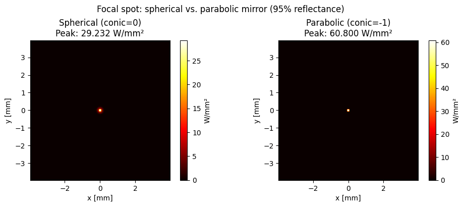
A spherical mirror (conic=0) suffers from spherical aberration for on-axis collimated input: marginal rays focus closer to the mirror than paraxial rays. A parabolic mirror (conic=-1) eliminates this aberration and focuses a collimated on-axis beam to a perfect geometrical point.

def mirror_spot(conic, aperture_radius=25, n_rays=40_000, reflectance=0.95):
    # Focal length = 100 mm (R = -200 mm, concave toward -z)
    scene_m = NSQScene()
    scene_m.add_source(
        'S', CoordinateSystem(z=-100),
        CollimatedSourceConfig(spec, total_flux=1.0, aperture_radius=aperture_radius),
    )
    scene_m.add_mirror(
        'M', CoordinateSystem(z=0),
        MirrorConfig(radius=-200, conic=conic, aperture_radius=aperture_radius + 2,
                     reflectance=reflectance),
    )
    scene_m.add_detector(
        'D', CoordinateSystem(z=-100),
        IrradianceDetectorConfig(width=8, height=8, num_pixels_x=128, num_pixels_y=128),
    )
    r = scene_m.trace(num_rays=n_rays, seed=42)
    return r.detectors['D']

irr_sphere  = mirror_spot(conic=0.0)
irr_parab   = mirror_spot(conic=-1.0)

fig, axes = plt.subplots(1, 2, figsize=(10, 4))
for ax, irr, title in zip(axes, [irr_sphere, irr_parab],
                          ['Spherical (conic=0)', 'Parabolic (conic=-1)']):
    im = ax.imshow(irr.irradiance, origin='lower', cmap='hot', aspect='equal',
                   extent=[irr.x_coords[0], irr.x_coords[-1],
                            irr.y_coords[0], irr.y_coords[-1]])
    plt.colorbar(im, ax=ax, label='W/mm²')
    ax.set_title(f'{title}\nPeak: {irr.irradiance.max():.3f} W/mm²')
    ax.set_xlabel('x [mm]'); ax.set_ylabel('y [mm]')
plt.suptitle('Focal spot: spherical vs. parabolic mirror (95% reflectance)', fontsize=12)
plt.tight_layout()
plt.show()
plt.close(fig)

3. Solar Concentrator

A parabolic dish captures parallel solar radiation and focuses it onto a small receiver. The concentration ratio is the peak receiver irradiance divided by the ambient solar irradiance.

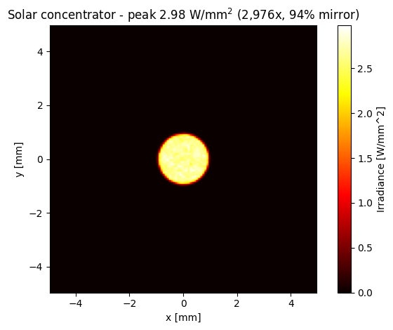
The physically important detail is that the Sun is not a point: it subtends about 0.53° from Earth, so a perfect parabola images it as a disc rather than a point, and that disc sets the achievable concentration. We model this with an ExtendedSource the size of the dish, in which every point emits into a ±0.265° cone.

The resulting spot radius should come out at f · tan(0.265°), the geometrical image of the solar disc. Concentration also scales directly with the dish’s reflectance — a real solar collector uses a silvered-glass or polished-metal mirror around 90-95% reflective, not the mathematical 100% a naive model would imply, so the concentration figure below already reflects that ~6% loss rather than overstating it.

# Solar irradiance ~ 1000 W/m^2 = 0.001 W/mm^2
mirror_radius = 50.0
solar_flux = 0.001 * np.pi * mirror_radius**2  # W intercepted by the dish
focal_length = 200.0  # f = |radius| / 2
dish_reflectance = 0.94  # typical second-surface silvered-glass solar mirror

# Broadband solar-like spectrum (visible + NIR)
spec_solar = Spectrum(
    wavelengths=np.array([0.4, 0.5, 0.6, 0.7, 0.8, 0.9, 1.0]),
    weights=np.array([0.6, 1.0, 1.1, 1.0, 0.9, 0.7, 0.5]),
)

scene_solar = NSQScene()
# The Sun: a disc of parallel-ish beams, each spread over the solar half-angle.
scene_solar.add_source(
    'Sun', CoordinateSystem(z=-200),
    ExtendedSourceConfig(spectrum=spec_solar, total_flux=solar_flux,
                         aperture_radius=mirror_radius,
                         half_angle_deg=0.265),   # solar disc half-angle
)
scene_solar.add_mirror(
    'Dish', CoordinateSystem(z=0),
    MirrorConfig(radius=-400, conic=-1.0, aperture_radius=mirror_radius + 2,
                 reflectance=dish_reflectance),
)
# Receiver at the focus (f = |radius| / 2 = 200 mm, on the -z side)
scene_solar.add_detector(
    'Receiver', CoordinateSystem(z=-focal_length),
    IrradianceDetectorConfig(width=10, height=10, num_pixels_x=128, num_pixels_y=128),
)

result_solar = scene_solar.trace(num_rays=120_000, seed=42)
irr_solar = result_solar.detectors['Receiver']

ambient = solar_flux / (np.pi * mirror_radius**2)
concentration = irr_solar.irradiance.max() / ambient

# Radius containing 90% of the collected flux
E = irr_solar.irradiance
X, Y = np.meshgrid(irr_solar.x_coords, irr_solar.y_coords)
R = np.hypot(X, Y)
order = np.argsort(R.ravel())
cumulative = np.cumsum(E.ravel()[order]) / E.sum()
r90 = R.ravel()[order][np.searchsorted(cumulative, 0.9)]
r_theory = focal_length * np.tan(np.radians(0.265))

print(f"Flux intercepted by dish : {solar_flux:.2f} W")
print(f"Mirror reflectance       : {dish_reflectance:.0%}")
print(f"Flux on receiver         : {irr_solar.total_flux:.3f} W "
      f"({irr_solar.total_flux / solar_flux * 100:.1f}% collected "
      f"of {dish_reflectance:.0%} available after the mirror)")
print(f"Peak concentration       : {concentration:,.0f}x ambient")
print(f"90% encircled radius     : {r90:.3f} mm")
print(f"Solar image radius       : {r_theory:.3f} mm  (f * tan(0.265 deg))")

fig = irr_solar.plot(cmap='hot')
plt.title(f'Solar concentrator - peak {irr_solar.irradiance.max():.2f} W/mm$^2$ '
          f'({concentration:,.0f}x, {dish_reflectance:.0%} mirror)')
plt.tight_layout()
plt.show()

Flux intercepted by dish : 7.85 W
Mirror reflectance       : 94%
Flux on receiver         : 7.383 W (94.0% collected of 94% available after the mirror)
Peak concentration       : 2,976x ambient
90% encircled radius     : 0.899 mm
Solar image radius       : 0.925 mm  (f * tan(0.265 deg))

4. Catadioptric System — Mirror + Lens

A catadioptric system combines a primary reflective element with a refractive corrector. Here we use a concave mirror as the primary and a singlet lens as a field-correcting relay.

scene_cat = NSQScene()
scene_cat.add_source(
    'S', CoordinateSystem(z=-150),
    CollimatedSourceConfig(spec, total_flux=1.0, aperture_radius=20.0),
)
# Primary mirror: f = 75 mm, 95% reflective (protected silver)
scene_cat.add_mirror(
    'PM', CoordinateSystem(z=0),
    MirrorConfig(radius=-150, conic=-1.0, aperture_radius=22.0, reflectance=0.95),
)
# Field corrector lens near the focus
scene_cat.add_lens(
    'FC', CoordinateSystem(z=-50),
    LensConfig(r1=-80, r2=80, thickness=4, material='N-BK7', front_aperture_radius=15.0),
)
# Detector
scene_cat.add_detector(
    'D', CoordinateSystem(z=-90),
    IrradianceDetectorConfig(width=8, height=8, num_pixels_x=128, num_pixels_y=128),
)

result_cat = scene_cat.trace(num_rays=50_000, seed=42)
irr_cat = result_cat.detectors['D']

fig = irr_cat.plot(cmap='hot')
plt.title(f'Catadioptric system | {irr_cat.num_rays_hit:,} rays on detector')
plt.tight_layout()
plt.show()
plt.close(fig)

# A nontrivial multi-surface trace like this one is exactly where it pays to
# check the self-diagnosing report before trusting the numbers above: it
# flags depth-truncated flux, Russian-roulette loss, and any component the
# trace never reached.
print(result_cat.report())

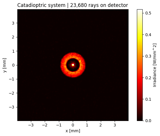
NSQ trace diagnostics:
  depth_truncated_flux_fraction: 0.0000%
  rr_killed_flux_fraction:       0.0000%
  flux_conservation_error:       4.2910%
  unreached_geometry:            none
  medium_stack_underflows:       0
  split_budget_saturated:        False
  detectors:
    D: 23680 hits, 1.45 mean hits/pixel [undersampled]
Warnings:
  - Detector 'D' is undersampled: 1.4 mean hits/pixel (< 10), shot noise dominates the map; ~13,837,837 rays would bring it to ~5% relative error.

5. Far-Field Radiation Pattern

A FarFieldDetector bins rays by direction rather than position, giving the angular distribution of the light leaving the system.

A point source exactly at the focus of a perfect parabola would collimate to zero divergence, which is not informative. A real emitter has finite size, and that size sets the divergence:

\[\theta_{\mathrm{FWHM}} \approx 2\arctan\left(\frac{r_{\mathrm{source}}}{f}\right)\]

Below, a 5 mm-radius emitter at the focus of a 100 mm parabola should give about 5.7° of divergence. This is the fundamental etendue trade: a bigger source cannot be collimated as tightly.

# Finite-size emitter at the focus of a parabolic collimator
led_radius = 5.0     # mm
focal_length = 100.0  # f = |radius| / 2 = 200 / 2

scene_farfield = NSQScene()
scene_farfield.add_source(
    'LED', CoordinateSystem(z=-focal_length),      # at the mirror focus
    ExtendedSourceConfig(spectrum=spec, total_flux=1.0,
                         aperture_radius=led_radius, half_angle_deg=90),
)
scene_farfield.add_mirror(
    'PM', CoordinateSystem(z=0),
    MirrorConfig(radius=-200, conic=-1.0, aperture_radius=30.0, reflectance=0.95),
)
# Fine theta bins: the beam is only a few degrees wide
scene_farfield.add_detector(
    'FF', CoordinateSystem(z=-150),
    FarFieldDetectorConfig(num_theta=180, num_phi=180),
)

result_ff = scene_farfield.trace(num_rays=150_000, seed=42)
ff = result_ff.detectors['FF']

# Azimuthally averaged radial profile
radial = ff.intensity.sum(axis=1)
profile = radial / radial.max()


def fwhm_deg(theta, profile):
    """Full width at half maximum, interpolated on the falling edge."""
    above = np.where(profile >= 0.5)[0]
    if len(above) < 2:
        return 0.0
    i = above[-1]
    if i + 1 < len(profile):
        frac = (profile[i] - 0.5) / (profile[i] - profile[i + 1])
        edge = theta[i] + frac * (theta[i + 1] - theta[i])
    else:
        edge = theta[i]
    return 2.0 * edge   # profile is symmetric about theta = 0


measured = fwhm_deg(ff.theta, profile)
predicted = 2.0 * np.degrees(np.arctan(led_radius / focal_length))

fig, ax = plt.subplots(figsize=(7, 4))
ax.plot(ff.theta, profile, lw=1.5)
ax.axhline(0.5, color='r', ls='--', lw=1,
           label=f'Half maximum (FWHM = {measured:.2f} deg)')
ax.axvline(predicted / 2, color='k', ls=':', lw=1,
           label=f'Predicted 2 arctan(r/f) = {predicted:.2f} deg')
ax.set_xlim(0, 15)
ax.set_xlabel('theta [deg]')
ax.set_ylabel('Normalised intensity')
ax.set_title('Far-field pattern: finite emitter + parabolic collimator')
ax.legend()
ax.grid(True, alpha=0.4)
plt.tight_layout()
plt.show()

print(f"Measured FWHM  : {measured:.2f} deg")
print(f"Predicted FWHM : {predicted:.2f} deg  (2 arctan(r_source / f))")

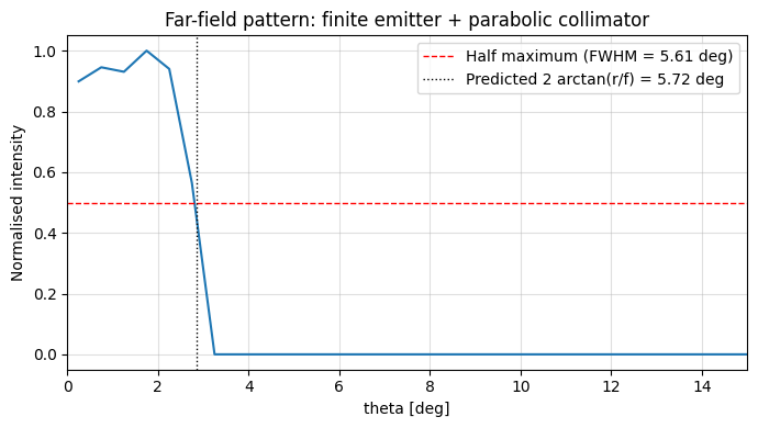
Measured FWHM  : 5.61 deg
Predicted FWHM : 5.72 deg  (2 arctan(r_source / f))

Summary

• MirrorConfig(radius, reflectance, conic, aperture_radius) — reflectance is required (a constant, a callable(wavelength_um), or a coating); there is no implicit 100%-reflector default, so every mirror in this notebook states a realistic value (0.94-0.95) rather than assuming a perfect one

• A mirror needs no rotation to face an incoming +z beam; the sign of radius sets whether it is concave (radius < 0 here) or convex

• Focal length of a mirror: f = |radius| / 2

• Parabolic mirrors eliminate on-axis spherical aberration for collimated input; spherical mirrors do not, and the residual blur grows with aperture

• Mix add_mirror and add_lens in the same scene for catadioptric systems

• FarFieldDetector measures beam divergence (FWHM) and angular distribution

• result.report() is worth a look after any multi-surface trace — it flags depth-truncated flux, Russian-roulette loss, and components the trace never reached, before you trust the numbers above them