Multi-Source Illumination

An NSQScene can hold any number of sources simultaneously. All sources launch rays in the same trace, and every ray carries flux proportional to its source’s total_flux. This makes it straightforward to model:

• Multi-point LED arrays — many PointSources at different positions

• Off-axis illumination — sources tilted relative to the optical axis

• Field uniformity analysis — sources spanning a range of field angles

• Mixed spectral sources — sources with different spectra

import matplotlib.pyplot as plt
import numpy as np

from optiland.coordinate_system import CoordinateSystem
from optiland.nonsequential import (
    NSQScene, Spectrum,
    PointSourceConfig, CollimatedSourceConfig, ExtendedSourceConfig,
    IrradianceDetectorConfig,
    LensConfig,
)

spec_w = Spectrum(wavelengths=np.array([0.45, 0.55, 0.65]),
                  weights=np.array([1.0, 1.0, 1.0]))
spec_green = Spectrum.monochromatic(0.55)

# Two lenses are reused throughout. Both are N-BK7 biconvex singlets; what
# matters for illumination work is where their focal points sit, so both
# prescriptions are reduced to numbers here once.
#
#   condenser  r1=40, r2=-40, t=5  ->  f = 39.41 mm, front focus z = -37.73
#   singlet    r1=50, r2=-50, t=5  ->  f = 49.05 mm, rear  focus z = +52.38
#
# A source placed at a lens's FRONT focal point leaves it collimated. That is
# the whole trick behind a condenser, and putting the source anywhere else is
# the most common reason an illumination model does not do what was intended.
CONDENSER = LensConfig(r1=40, r2=-40, thickness=5, material='N-BK7',
                       front_aperture_radius=15.0)
CONDENSER_FRONT_FOCUS = -37.73

SINGLET = LensConfig(r1=50, r2=-50, thickness=5, material='N-BK7',
                     front_aperture_radius=15.0)
SINGLET_REAR_FOCUS = 52.38

1. LED Array — Multiple PointSources

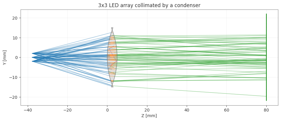
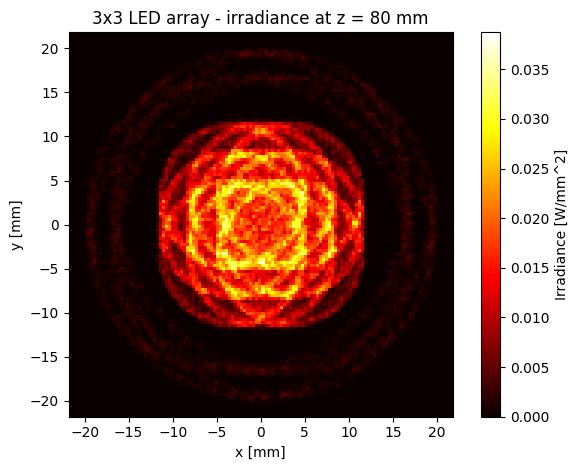
Model a 3×3 LED array with 2 mm pitch. Each LED is a PointSource with a narrow emission cone. (A true Lambertian die would emit over the full hemisphere with cosine weighting; ExtendedSourceConfig models that case, and a finite die size as well.)

Two numbers decide whether this scene means anything.

Where the array sits. To collimate the array the LEDs go at the condenser’s front focal point, z = −37.73 mm. Each LED then leaves the lens as its own collimated bundle, tilted by atan(x / f) — 2.9° for the outermost LEDs at ±2 mm. Put the array at z = −20 instead, well inside the focal length, and the lens forms a virtual image: the light still diverges and nothing is collimated, whatever the comment says.

How wide the cone is. From 37.73 mm away, the 15 mm lens semi-diameter subtends atan(15 / 37.73) = 21.7°. A 20° half-angle fills the aperture without spilling much light past the glass — rays that miss the lens reach the detector unfocused and quietly corrupt the uniformity numbers computed in the next section.

pitch = 2.0  # mm between LEDs
scene_array = NSQScene()

# 3x3 grid of LEDs at the condenser's front focal plane
for i, x in enumerate(np.linspace(-pitch, pitch, 3)):
    for j, y in enumerate(np.linspace(-pitch, pitch, 3)):
        scene_array.add_source(
            f'LED_{i}_{j}',
            CoordinateSystem(x=x, y=y, z=CONDENSER_FRONT_FOCUS),
            PointSourceConfig(
                spectrum=spec_w, total_flux=1.0, half_angle_deg=20,
            ),
        )

# Condenser lens: collimates each LED into its own tilted bundle
scene_array.add_lens('L', CoordinateSystem(z=0), CONDENSER)

# Detector in the collimated space downstream of the condenser
scene_array.add_detector(
    'D', CoordinateSystem(z=80),
    IrradianceDetectorConfig(width=44, height=44, num_pixels_x=128, num_pixels_y=128),
)

result_array = scene_array.trace(num_rays=90_000, seed=42)
irr_array = result_array.detectors['D']

print(f"Total sources    : {len(scene_array.sources)}")
print(f"Total flux in    : {result_array.total_flux_in:.2f} W")
print(f"Flux detected    : {irr_array.total_flux:.3f} W "
      f"({100 * irr_array.total_flux / result_array.total_flux_in:.0f}% collected)")
print(f"Flux escaped     : {result_array.total_flux_escaped:.3f} W")

scene_array.view(num_rays=80, color_by='bounce',
                 title='3x3 LED array collimated by a condenser')
plt.show()

fig = irr_array.plot(cmap='hot')
plt.title('3x3 LED array - irradiance at z = 80 mm')
plt.tight_layout()
plt.show()
plt.close(fig)

Total sources    : 9
Total flux in    : 9.00 W
Flux detected    : 7.617 W (85% collected)
Flux escaped     : 1.368 W

2. Illumination Uniformity Analysis

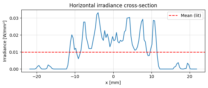
A key figure of merit for illumination systems is uniformity — how evenly the flux is distributed across the target. Common metrics:

• Uniformity ratio = min / max irradiance

• RMS uniformity = 1 − σ / μ

• ±X% area = fraction of pixels within X% of the mean

All of them are computed over the lit region, so they are only as meaningful as the definition of “lit”. The 1%-of-peak threshold used below is a convention, not a law; a scene where stray unfocused light reaches the detector will drag the threshold down and flatter the numbers.

E = irr_array.irradiance
# Only consider lit pixels (above 1% of peak)
lit = E > 0.01 * E.max()
E_lit = E[lit]

uniformity_min_max = E_lit.min() / E_lit.max()
rms_uniformity     = 1.0 - E_lit.std() / E_lit.mean()
within_20pct       = np.mean(np.abs(E_lit - E_lit.mean()) < 0.20 * E_lit.mean()) * 100

print(f"Uniformity (min/max)  : {uniformity_min_max:.3f}")
print(f"RMS uniformity (1-σ/μ): {rms_uniformity:.3f}")
print(f"Pixels within ±20% μ  : {within_20pct:.1f}%")

# Horizontal profile
ny, nx = E.shape
row_centre = E[ny // 2, :]

fig, ax = plt.subplots(figsize=(7, 3))
ax.plot(irr_array.x_coords, row_centre)
ax.axhline(row_centre.mean(), color='r', linestyle='--', label='Mean (lit)')
ax.set_xlabel('x [mm]')
ax.set_ylabel('Irradiance [W/mm²]')
ax.set_title('Horizontal irradiance cross-section')
ax.legend()
ax.grid(True, alpha=0.4)
plt.tight_layout()
plt.show()
plt.close(fig)

Uniformity (min/max)  : 0.010
RMS uniformity (1-σ/μ): -0.026
Pixels within ±20% μ  : 7.2%

3. Off-Axis and Tilted Sources

Tilt a source by setting rx and ry in the CoordinateSystem (values in radians). This lets you model off-axis field angles or oblique illumination.

scene_tilt = NSQScene()

# On-axis source
scene_tilt.add_source(
    'S_on', CoordinateSystem(z=-80),
    CollimatedSourceConfig(spectrum=spec_green, total_flux=1.0, aperture_radius=8.0),
)
# 5-degree tilted source (field angle)
scene_tilt.add_source(
    'S_off', CoordinateSystem(z=-80, rx=np.radians(5)),
    CollimatedSourceConfig(spectrum=spec_green, total_flux=1.0, aperture_radius=8.0),
)

scene_tilt.add_lens('L', CoordinateSystem(z=0), SINGLET)

# Both sources are collimated, so both focus at the rear focal plane. The
# tilted one lands off axis at -f*tan(5 deg) = -4.3 mm; that separation is the
# whole point of the figure, and it vanishes into a common blur if the
# detector is anywhere else.
scene_tilt.add_detector(
    'D', CoordinateSystem(z=SINGLET_REAR_FOCUS),
    IrradianceDetectorConfig(width=16, height=16, num_pixels_x=192, num_pixels_y=192),
)

result_tilt = scene_tilt.trace(num_rays=120_000, seed=42)
irr_tilt = result_tilt.detectors['D']

fig = irr_tilt.plot(cmap='hot')
plt.axhline(0.0, color='cyan', lw=0.6, ls=':')
plt.axhline(-49.05 * np.tan(np.radians(5)), color='cyan', lw=0.6, ls=':')
plt.title('On-axis + 5\u00b0 off-axis collimated sources, at the focal plane')
plt.tight_layout()
plt.show()
plt.close(fig)

print(f"Predicted off-axis spot: y = -f*tan(5\u00b0) = "
      f"{-49.05 * np.tan(np.radians(5)):+.2f} mm")

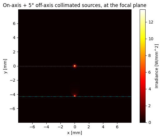
Predicted off-axis spot: y = -f*tan(5°) = -4.29 mm

4. Mixed-Spectrum Sources

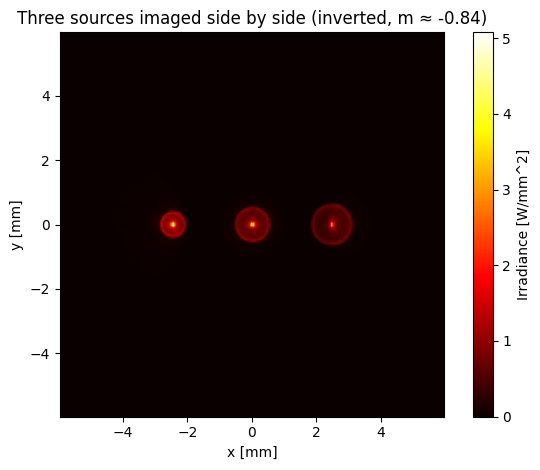
Each source can have an independent Spectrum. Here three point sources at different wavelengths and different heights are imaged by the singlet.

Placing them 100 mm in front of the lens — roughly twice the focal length — puts the image near z = 87 mm at a magnification of about −0.84, so the three sources arrive as three resolved, inverted spots.

One caveat worth stating plainly: an IrradianceMap records total flux per pixel, with no wavelength axis. It cannot show colour. To separate the three wavelengths you need a SpectralDetector, which bins flux by wavelength — see notebook 04.

spec_r = Spectrum.monochromatic(0.64)   # red
spec_g = Spectrum.monochromatic(0.532)  # green
spec_b = Spectrum.monochromatic(0.45)   # blue

scene_rgb = NSQScene()

# Three point sources at 3 mm separation, each a different colour. The 8-degree
# cone fills the 15 mm lens from 100 mm away without spilling past it.
for name, spec, x in [('R', spec_r, -3.0), ('G', spec_g, 0.0), ('B', spec_b, 3.0)]:
    scene_rgb.add_source(
        name, CoordinateSystem(x=x, z=-100),
        PointSourceConfig(spectrum=spec, total_flux=1.0, half_angle_deg=8),
    )

scene_rgb.add_lens('L', CoordinateSystem(z=0), SINGLET)
scene_rgb.add_detector(
    'D', CoordinateSystem(z=87),
    IrradianceDetectorConfig(width=12, height=12, num_pixels_x=192, num_pixels_y=192),
)

result_rgb = scene_rgb.trace(num_rays=120_000, seed=42)
irr_rgb = result_rgb.detectors['D']

fig = irr_rgb.plot(cmap='hot')
plt.title('Three sources imaged side by side (inverted, m \u2248 -0.84)')
plt.tight_layout()
plt.show()
plt.close(fig)

print(f"Total flux in    : {result_rgb.total_flux_in:.4f} W  (3 sources \u00d7 1 W each)")
print(f"Flux on detector : {irr_rgb.total_flux:.4f} W")
print("\nSource x = -3.0, 0.0, +3.0 mm  ->  image x \u2248 +2.5, 0.0, -2.5 mm")

Total flux in    : 3.0000 W  (3 sources × 1 W each)
Flux on detector : 2.5772 W

Source x = -3.0, 0.0, +3.0 mm  ->  image x ≈ +2.5, 0.0, -2.5 mm

5. Extended Source for Diffuse Illumination

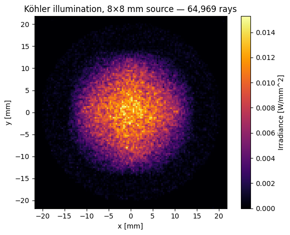
An ExtendedSource uniformly samples positions on a rectangle. Put it at the condenser’s front focal plane and you have Köhler illumination: the source is imaged to infinity, so the target sees an even wash of light rather than a picture of the emitter.

The same aperture-filling rule applies. The original 45° cone from 50 mm away would have thrown a 50 mm beam radius at a lens with a 15 mm semi-diameter, sending roughly nine tenths of the light past the glass and onto the detector as unfocused spill.

scene_ext = NSQScene()
scene_ext.add_source(
    'ES', CoordinateSystem(z=CONDENSER_FRONT_FOCUS),
    ExtendedSourceConfig(
        spectrum=spec_green, total_flux=5.0,
        width=8, height=8, half_angle_deg=20,
    ),
)
scene_ext.add_lens('L', CoordinateSystem(z=0), CONDENSER)
scene_ext.add_detector(
    'D', CoordinateSystem(z=80),
    IrradianceDetectorConfig(width=44, height=44, num_pixels_x=128, num_pixels_y=128),
)

result_ext = scene_ext.trace(num_rays=80_000, seed=0)
irr_ext = result_ext.detectors['D']

E_ext = irr_ext.irradiance
lit_ext = E_ext > 0.01 * E_ext.max()
print(f"Collected: {irr_ext.total_flux:.3f} W of {result_ext.total_flux_in:.1f} W "
      f"({100 * irr_ext.total_flux / result_ext.total_flux_in:.0f}%)")
print(f"RMS uniformity over the lit area: "
      f"{1 - E_ext[lit_ext].std() / E_ext[lit_ext].mean():.3f}")

fig = irr_ext.plot(cmap='inferno')
plt.title(f'K\u00f6hler illumination, 8\u00d78 mm source \u2014 {irr_ext.num_rays_hit:,} rays')
plt.tight_layout()
plt.show()
plt.close(fig)

Collected: 4.055 W of 5.0 W (81%)
RMS uniformity over the lit area: -0.034

Summary

• Add as many sources as needed — all participate in the same trace

• Source position: CoordinateSystem(x, y, z) in mm

• Source tilt: CoordinateSystem(rx=..., ry=...) in radians

• Each source can have an independent Spectrum and total_flux

• total_flux_in in SimulationResult sums across all sources

• Analyse uniformity via irradiance.min/max/std/mean on the IrradianceMap

Two habits carry across every illumination model in this notebook:

• Match the source cone to the aperture. Light that misses the optic still reaches the detector, where it inflates the collected flux and corrupts every uniformity metric computed from the map.

• Place sources and detectors by the prescription, not by eye. A condenser collimates only from its front focal point; a collimated beam focuses only at the rear focal plane. Check total_flux_escaped and flux_conservation_error before trusting any number that comes out.