Radiant Intensity

optiland.analysis.RadiantIntensity groups traced rays by their outgoing direction, rather than by where they hit the image plane. This example uses the on-axis field of the Cooke triplet at its primary wavelength (0.55 µm).

We use relative mode: the stored map contains summed ray weights per angular bin, and the plots are normalized to their peak. These weights are not calibrated power, so this example does not report W/sr. Absolute radiant intensity requires ray powers in watts and use_absolute_units=True, which also divides each bin’s power by its solid angle.

from io import BytesIO

import matplotlib.pyplot as plt
from IPython.display import Image, display

from optiland.analysis import RadiantIntensity
from optiland.samples.objectives import CookeTriplet


def show_figure(fig):
    """Embed a figure even when running with MPLBACKEND=Agg."""
    buffer = BytesIO()
    fig.savefig(buffer, format="png", dpi=120, bbox_inches="tight")
    display(Image(data=buffer.getvalue()))
    plt.close(fig)


lens = CookeTriplet()

Choose the angular window and sampling

reference_surface_index=-1 uses directions at the image surface. X and Y angles are the projections atan2(L, N) and atan2(M, N), in degrees, where L, M and N are direction cosines.

They are not positions in millimeters or the polar and azimuthal angles of spherical coordinates. X angle is the angle between the ray’s projection and the Z axis in the XZ plane, and Y angle is the angle between the ray’s projection and the Z axis in the YZ plane.

The window below covers −8° to +8° in both directions. Rays outside that window are not binned. More bins reveal finer structure but require more rays to avoid sparse bins. For distribution="hexapolar", num_rays=80 means 80 pupil rings, not 80 individual rays: the deterministic pattern contains 19,441 launch points.

intensity = RadiantIntensity(
    lens,
    fields=[(0.0, 0.0)],
    wavelengths="primary",
    distribution="hexapolar",
    num_rays=80,
    reference_surface_index=-1,
    num_angular_bins_X=41,
    num_angular_bins_Y=31,
    angle_X_min=-8.0,
    angle_X_max=8.0,
    angle_Y_min=-8.0,
    angle_Y_max=8.0,
    use_absolute_units=False,
)

Read the map and central profile

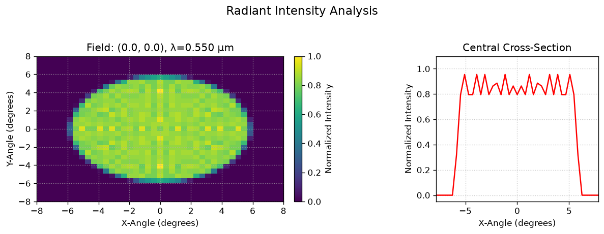
The color represents the summed weight in each angular bin divided by the largest bin weight in this field/wavelength map. The peak is 1; a value of 0.5 means half the peak bin weight, not half the total power. Empty bins have value zero. The right-hand curve is the X-angle profile through the central Y-angle bin.

In relative mode, normalize=True changes only the display: intensity.data still holds unnormalized bin weights. Sampling and bin size affect the pattern; it is not an image-plane irradiance map or a calibrated per-steradian distribution.

fig, axes = intensity.view(normalize=True, cmap="viridis", figsize=(10, 4), show=False)
fig.subplots_adjust(wspace=0.6)
show_figure(fig)

Select a different cross-section

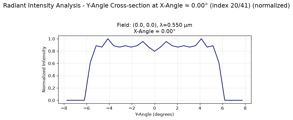
cross_section=("cross-y", -1) plots Y angle at the central X-angle bin; −1 selects the central bin. Use ("cross-x", index) to select a fixed Y-angle bin instead. Normalization still uses the peak of the whole map, so an arbitrary slice need not reach 1.

fig, axes = intensity.view(
    cross_section=("cross-y", -1),
    normalize=True,
    cross_section_color="navy",
    figsize=(7, 4),
    show=False,
)
show_figure(fig)