
Tutorial 3f: Constrained Optimization with the Default Merit#
November 2026#
An unconstrained optimizer is happy to produce a lens that cannot be made: an element that thins to nothing, or an edge with negative thickness. This tutorial builds a realistic design problem with three tools that keep things short and safe:
problem.add_default_merit(...): a spot-size merit function in one call, using a few well-chosen pupil rays (Gaussian quadrature).problem.add_physical_constraints(...): thickness limits that the optimizer must obey (hard constraints).minimize(problem, "dls"): the native damped least-squares optimizer, with an observer that records the run and a token that can cancel it.
The background is in the Optimization Guide and Default Merit and Constraints.
[1]:
import matplotlib.pyplot as plt
import numpy as np

import optiland.backend as be
from optiland.optimization import (
    CancelToken,
    DefaultMeritBlock,
    HistoryObserver,
    OptimizationProblem,
    minimize,
)
from optiland.optimization.operand.lens import LensOperand
from optiland.samples.objectives import CookeTriplet
A starting design#
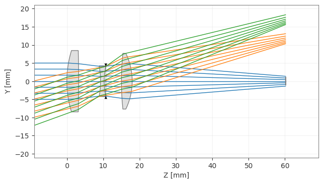
We take the Optiland Cooke triplet and disturb its radii by about 15 % (with a fixed seed) so that there is real work to do. The focal length of the original is 50 mm.
[2]:
def starting_lens():
    lens = CookeTriplet()
    rng = np.random.default_rng(3)
    for k in range(1, 7):
        geometry = lens.surfaces[k].geometry
        geometry.radius = geometry.radius * (1 + 0.15 * rng.standard_normal())
    return lens


lens = starting_lens()
lens.draw(num_rays=7)
[2]:
(<Figure size 1000x400 with 1 Axes>, <Axes: xlabel='Z [mm]', ylabel='Y [mm]'>)
The default merit#
add_default_merit adds one block of per-ray residuals instead of one operand per number. With rings=3, arms=6 it traces 18 rays for every field and wavelength; each ray carries a quadrature weight, so sum(r**2) estimates the weighted RMS spot size squared. reference="centroid" measures spots from their centroid (and from the primary-wavelength centroid for other wavelengths, so lateral color counts).
We keep an ordinary operand for the focal length: blocks and operands mix freely. We let all radii and the air and glass thicknesses vary, with a small lower bound on thickness.
[3]:
def make_problem(lens, constrained):
    problem = OptimizationProblem()

    problem.add_default_merit(lens, kind="spot", rings=3, arms=6)
    problem.add_operand("f2", target=50.0, weight=10.0, input_data={"optic": lens})

    num_surfaces = lens.surfaces.num_surfaces
    for k in range(1, num_surfaces - 1):
        problem.add_variable(lens, "radius", surface_number=k)
    for k in range(1, num_surfaces - 2):
        problem.add_variable(lens, "thickness", surface_number=k, min_val=0.1)

    if constrained:
        problem.add_physical_constraints(
            lens,
            min_center_glass=2.0,
            min_edge_glass=1.0,
            min_center_air=0.5,
            max_center=15.0,
        )
    return problem


free_lens = starting_lens()
free_problem = make_problem(free_lens, constrained=False)
free_problem.info()
╒════╤════════════════════════╤═══════════════════╕
│    │   Merit Function Value │   Improvement (%) │
╞════╪════════════════════════╪═══════════════════╡
│  0 │                11059.7 │                 0 │
╘════╧════════════════════════╧═══════════════════╛
╒════╤════════════════╤══════════╤══════════════╤══════════════╤══════════╤═══════════════╤═════════╤═════════╤════════════════╕
│    │ Operand Type   │   Target │ Min. Bound   │ Max. Bound   │   Weight │   Eff. Weight │   Value │   Delta │   Contrib. [%] │
╞════╪════════════════╪══════════╪══════════════╪══════════════╪══════════╪═══════════════╪═════════╪═════════╪════════════════╡
│  0 │ f2             │       50 │              │              │       10 │            10 │  60.513 │  10.513 │          99.93 │
╘════╧════════════════╧══════════╧══════════════╧══════════════╧══════════╧═══════════════╧═════════╧═════════╧════════════════╛
╒════╤═══════════════════╤════════╤═════════════╤══════════╤═══════════════╤════════╤══════════╤════════╤═══════════╤═════════╤════════════════╕
│    │ Block             │ Kind   │ Reference   │   Fields │   Wavelengths │   Rays │   Weight │   Rows │   Dropped │   Merit │   Contrib. [%] │
╞════╪═══════════════════╪════════╪═════════════╪══════════╪═══════════════╪════════╪══════════╪════════╪═══════════╪═════════╪════════════════╡
│  0 │ DefaultMeritBlock │ spot   │ centroid    │        3 │             3 │    162 │        1 │    324 │         0 │ 8.06123 │           0.07 │
╘════╧═══════════════════╧════════╧═════════════╧══════════╧═══════════════╧════════╧══════════╧════════╧═══════════╧═════════╧════════════════╛
╒════╤═════════════════╤═══════════╤════════════╤══════════════╤══════════════╕
│    │ Variable Type   │   Surface │      Value │   Min. Bound │ Max. Bound   │
╞════╪═════════════════╪═══════════╪════════════╪══════════════╪══════════════╡
│  0 │ radius          │         1 │   28.7528  │        nan   │              │
│  1 │ radius          │         2 │ -268.712   │        nan   │              │
│  2 │ radius          │         3 │  -23.6064  │        nan   │              │
│  3 │ radius          │         4 │   18.5637  │        nan   │              │
│  4 │ radius          │         5 │   74.2733  │        nan   │              │
│  5 │ radius          │         6 │  -17.8004  │        nan   │              │
│  6 │ thickness       │         1 │    3.25896 │          0.1 │              │
│  7 │ thickness       │         2 │    6.00755 │          0.1 │              │
│  8 │ thickness       │         3 │    0.99997 │          0.1 │              │
│  9 │ thickness       │         4 │    4.75041 │          0.1 │              │
│ 10 │ thickness       │         5 │    2.95208 │          0.1 │              │
╘════╧═════════════════╧═══════════╧════════════╧══════════════╧══════════════╛
The first table is the operand (f2), the second the default-merit block: one summary row for 324 residuals (3 fields × 3 wavelengths × 18 rays × 2 coordinates).
Run 1: no constraints#
minimize with method="dls" is the native damped least-squares optimizer. A HistoryObserver records the merit after every accepted step. Note that minimize changes the lens in place.
[4]:
free_history = HistoryObserver()
free_result = minimize(free_problem, "dls", observers=[free_history])

print(free_result.stop_reason)
print(f"merit {free_problem.sum_squared():.3e}   residual evaluations {free_result.n_evals}")
`ftol` termination condition is satisfied.
merit 7.761e-04   residual evaluations 229
Image quality is excellent, but look at the glass. The table lists the center and edge thickness of every gap between surfaces (gap k lies after surface k):
[5]:
def thickness(operand, lens, k):
    return float(np.ravel(be.to_numpy(operand(lens, k)))[0])


def thickness_table(lens):
    print(" gap   center    edge")
    for k in range(1, lens.surfaces.num_surfaces - 2):
        center = thickness(LensOperand.center_thickness, lens, k)
        edge = thickness(LensOperand.edge_thickness, lens, k)
        flag = "   <-- not buildable" if edge < 0 or center < 0.5 else ""
        print(f"  {k}   {center:7.3f} {edge:7.3f}{flag}")


thickness_table(free_lens)
 gap   center    edge
  1     4.376   2.347
  2     5.384   4.038
  3     0.100   0.830   <-- not buildable
  4     5.449   4.497
  5     0.100  -1.614   <-- not buildable
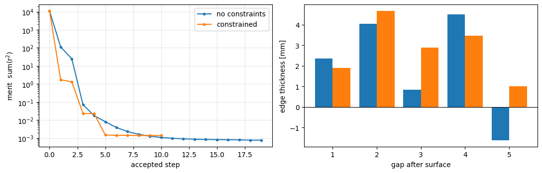
Some gaps have shrunk to the 0.1 mm bound and an edge thickness is negative: the surfaces cross each other at the rim. The optimizer exploited the freedom we gave it.
Run 2: physical constraints#
add_physical_constraints places limits on every gap between lens surfaces in one call. In the default mode="constraint" they are hard constraints: they are not in the merit, and the optimizer must satisfy them. The gaps from the object and to the image are never limited. Let us build the same problem, with limits, from the same starting design.
[6]:
lens = starting_lens()
problem = make_problem(lens, constrained=True)
problem.constraint_info()
╒════╤════════════════════════════╤════════════╤═══════════════╤════════════╤═════════════╤════════════╕
│    │ Constraint                 │ Kind       │   Eff. Weight │   Residual │   Violation │ Feasible   │
╞════╪════════════════════════════╪════════════╪═══════════════╪════════════╪═════════════╪════════════╡
│  0 │ #0 center_thickness >= 2   │ inequality │             1 │    -1.259  │      0      │ True       │
│  1 │ #1 center_thickness <= 15  │ inequality │             1 │   -11.74   │      0      │ True       │
│  2 │ #2 edge_thickness >= 1     │ inequality │             1 │    -0.6939 │      0      │ True       │
│  3 │ #3 center_thickness >= 0.5 │ inequality │             1 │    -5.508  │      0      │ True       │
│  4 │ #4 center_thickness <= 15  │ inequality │             1 │    -8.992  │      0      │ True       │
│  5 │ #5 center_thickness >= 2   │ inequality │             1 │     1      │      1      │ False      │
│  6 │ #6 center_thickness <= 15  │ inequality │             1 │   -14      │      0      │ True       │
│  7 │ #7 edge_thickness >= 1     │ inequality │             1 │    -0.9175 │      0      │ True       │
│  8 │ #8 center_thickness >= 0.5 │ inequality │             1 │    -4.25   │      0      │ True       │
│  9 │ #9 center_thickness <= 15  │ inequality │             1 │   -10.25   │      0      │ True       │
│ 10 │ #10 center_thickness >= 2  │ inequality │             1 │    -0.9521 │      0      │ True       │
│ 11 │ #11 center_thickness <= 15 │ inequality │             1 │   -12.05   │      0      │ True       │
│ 12 │ #12 edge_thickness >= 1    │ inequality │             1 │     0.2103 │      0.2103 │ False      │
╘════╧════════════════════════════╧════════════╧═══════════════╧════════════╧═════════════╧════════════╛
Each limit is a row with its current residual and whether it is satisfied. The starting design violates some of them; the optimizer first restores feasibility.
[7]:
history = HistoryObserver()
result = minimize(problem, "dls", observers=[history])

print(result.stop_reason)
print(f"merit {problem.sum_squared():.3e}   residual evaluations {result.n_evals}")
print(f"success: {result.success}   max violation: {result.max_constraint_violation:.1e}")
thickness_table(lens)
`ftol` termination condition is satisfied.
merit 1.398e-03   residual evaluations 135
success: True   max violation: 3.3e-15
 gap   center    edge
  1     3.770   1.890
  2     5.991   4.671
  3     2.000   2.891
  4     4.273   3.474
  5     3.138   1.000
Every gap now respects its limit. The price is a higher merit than run 1 (about twice as large here): the unconstrained result was only that good because it was not buildable. The result also tells us which constraints are binding, and how much they cost:
[8]:
problem.constraint_info()
for label in result.active_set:
    print(f"binding: {label:30s} multiplier {result.multipliers[label]:.2e}")
╒════╤════════════════════════════╤════════════╤═══════════════╤═════════════╤═════════════╤════════════╕
│    │ Constraint                 │ Kind       │   Eff. Weight │    Residual │   Violation │ Feasible   │
╞════╪════════════════════════════╪════════════╪═══════════════╪═════════════╪═════════════╪════════════╡
│  0 │ #0 center_thickness >= 2   │ inequality │             1 │  -1.77      │   0         │ True       │
│  1 │ #1 center_thickness <= 15  │ inequality │             1 │ -11.23      │   0         │ True       │
│  2 │ #2 edge_thickness >= 1     │ inequality │             1 │  -0.8904    │   0         │ True       │
│  3 │ #3 center_thickness >= 0.5 │ inequality │             1 │  -5.491     │   0         │ True       │
│  4 │ #4 center_thickness <= 15  │ inequality │             1 │  -9.009     │   0         │ True       │
│  5 │ #5 center_thickness >= 2   │ inequality │             1 │  -0         │   0         │ True       │
│  6 │ #6 center_thickness <= 15  │ inequality │             1 │ -13         │   0         │ True       │
│  7 │ #7 edge_thickness >= 1     │ inequality │             1 │  -1.891     │   0         │ True       │
│  8 │ #8 center_thickness >= 0.5 │ inequality │             1 │  -3.773     │   0         │ True       │
│  9 │ #9 center_thickness <= 15  │ inequality │             1 │ -10.73      │   0         │ True       │
│ 10 │ #10 center_thickness >= 2  │ inequality │             1 │  -1.138     │   0         │ True       │
│ 11 │ #11 center_thickness <= 15 │ inequality │             1 │ -11.86      │   0         │ True       │
│ 12 │ #12 edge_thickness >= 1    │ inequality │             1 │   3.331e-15 │   3.331e-15 │ True       │
╘════╧════════════════════════════╧════════════╧═══════════════╧═════════════╧═════════════╧════════════╛
binding: #5 center_thickness >= 2       multiplier 1.75e-04
binding: #12 edge_thickness >= 1        multiplier 1.18e-04
A binding constraint with a large multiplier is a good candidate to relax: loosening it would improve the merit the most.
Let us compare the two runs.
[9]:
fig, axes = plt.subplots(1, 2, figsize=(11, 3.6))
for name, hist in (("no constraints", free_history), ("constrained", history)):
    axes[0].semilogy(
        [r["iteration"] for r in hist.records], [r["value"] for r in hist.records],
        marker="o", ms=3, label=name,
    )
axes[0].set_xlabel("accepted step")
axes[0].set_ylabel("merit  sum(r$^2$)")
axes[0].legend()
axes[0].grid(True, alpha=0.3)

for k in range(1, lens.surfaces.num_surfaces - 2):
    axes[1].bar(
        [k - 0.2, k + 0.2],
        [thickness(LensOperand.edge_thickness, free_lens, k),
         thickness(LensOperand.edge_thickness, lens, k)],
        width=0.4, color=["tab:blue", "tab:orange"],
    )
axes[1].axhline(0, color="k", lw=0.8)
axes[1].set_xlabel("gap after surface")
axes[1].set_ylabel("edge thickness [mm]")
fig.tight_layout()
plt.show()
[10]:
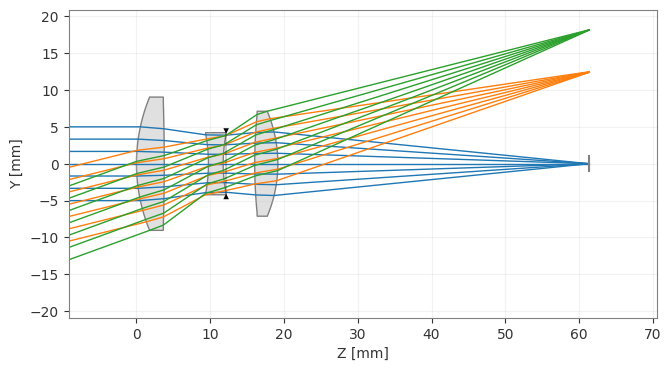
lens.draw(num_rays=7)
[10]:
(<Figure size 1000x400 with 1 Axes>, <Axes: xlabel='Z [mm]', ylabel='Y [mm]'>)
Watching and cancelling a run#
An observer is any object with on_start, on_step and on_end methods, and a CancelToken stops a run cleanly from anywhere (a button, a timer, another thread). Here an observer cancels the run after three accepted steps. The lens keeps the best design reached so far.
[11]:
class StopAfter:
    def __init__(self, token, steps):
        self.token, self.steps = token, steps

    def on_start(self, state):
        print("start: merit", f"{state.value:.3e}")

    def on_step(self, state):
        print(f"step {state.iteration}: merit {state.value:.3e}  evaluations {state.n_evals}")
        if state.iteration >= self.steps:
            self.token.cancel()

    def on_end(self, state, result):
        print("end:", result.stop_reason)


cancel_lens = starting_lens()
cancel_problem = make_problem(cancel_lens, constrained=True)
token = CancelToken()
cancelled = minimize(
    cancel_problem, "dls", observers=[StopAfter(token, 3)], cancel_token=token
)
start: merit 1.106e+04
step 1: merit 1.715e+00  evaluations 13
step 2: merit 1.308e+00  evaluations 26
step 3: merit 2.326e-02  evaluations 38
end: Stopped by a stopping criterion: cancelled by user.
For quick progress output, minimize(problem, "dls", disp=True) attaches a ConsoleObserver.
How many rays does the merit need?#
Gaussian quadrature uses few rays because it is an integral rule, not a sample. We can check the choice on the final design by building the merit with more rings and arms: if the value barely moves, three rings were enough.
[12]:
for rings, arms in [(2, 6), (3, 6), (4, 8), (6, 12)]:
    check = OptimizationProblem()
    check.add_residual_block(DefaultMeritBlock(lens, "spot", rings=rings, arms=arms))
    print(f"rings={rings}, arms={arms:2d}:  sum(r^2) = {check.sum_squared():.4e}")
rings=2, arms= 6:  sum(r^2) = 1.3849e-03
rings=3, arms= 6:  sum(r^2) = 1.3983e-03
rings=4, arms= 8:  sum(r^2) = 1.3835e-03
rings=6, arms=12:  sum(r^2) = 1.3837e-03
Summary and where to go next#
Task |
Call |
|---|---|
Spot or wavefront merit in one call |
|
Manufacturing limits on thickness |
|
Any other hard limit |
|
Run, watch and cancel |
|
Hard constraints are enforced by "dls" only; other optimizers raise an error rather than ignore them. If you need another optimizer, use mode="penalty" instead (see Default Merit and Constraints). For method selection, speed tips and failure behavior, see the Optimization Guide.