
Tutorial 8a: Custom Surface Types#
This tutorial shows how new surface types can be defined and used in Optiland. In general, any surface geometry can be defined in Optiland, so long as the surface equation is defined and it is differentiable.
To demonstrate this, we will generate a new surface that is defined by the following equation:
\(z(x, y) = \frac{r^2}{R \cdot (1 + \sqrt{(1 - (1 + k) \cdot r^2 / R^2)})} + ar + br^3 + c\sin(dr^2)\)
where
\(x\) and \(y\) are the local surface coordinates
\(r = \sqrt{x^2 + y^2}\)
\(R\) is the radius of curvature
\(k\) is the conic constant
\(a\), \(b\), \(c\) and \(d\) are coefficients
In this tutorial, we will generate a simple singlet lens whose first surface is defined by this equation.
[1]:
import warnings

import matplotlib.pyplot as plt
import numpy as np

from optiland import optic
from optiland.coordinate_system import CoordinateSystem
from optiland.geometries import NewtonRaphsonGeometry
from optiland.materials import IdealMaterial, Material
from optiland.surfaces import Surface
Introduction
In Optiland, an optic is defined as a collection of sequential surfaces. Each surface can be defined by the following components
Geometry - the physical shape of the surface
Material (pre-surface) - the material before the surface
Material (post-surface) - the material after the surface
Physical aperture - optionally, we can specify obscurations on the surface, such as a hole in the surface center.
Interaction model - defines how rays interact with the surface and includes properties like:
Whether surface is reflective, refractive, diffractive, or has some other behavior
Coating - a coating can be applied to the surface
Scatter model - a scatter model can be applied to the surface.
In general, we also specify whether the surface is the aperture stop.
In this tutorial, we will focus on only the geometry component.
Geometry Definition
To create our custom surface, we will need to create a new geometry class that uses the surface equation defined above.
We will start by inheriting from the “NewtonRaphsonGeometry” class. This class uses the Newton-Raphson method to find ray intersection points on the surface. We simply need to define the surface sag equation (from above) and the equation for the surface normal. Every geometry requires at least a coordinate system input, but we also want to include arguments for the radius of curvature, conic constant, and the coefficients.
We define the surface equation in the “sag” method and we define the surface normal in the “_surface_normal” method. Determining the surface normal involves finding the gradient of the surface equation:
\(f(x, y, z) = 0 = \frac{r^2}{R \cdot (1 + \sqrt{(1 - (1 + k) \cdot r^2 / R^2)})} + ar + br^3 + c\sin(dr^2) - z\)
[2]:
class NewGeometry(NewtonRaphsonGeometry):
    def __init__(self, coordinate_system, radius, conic, a, b, c, d):
        super().__init__(coordinate_system, radius, conic=conic, tol=1e-10, max_iter=100)
        self.a = a
        self.b = b
        self.c = c
        self.d = d

    def sag(self, x=0, y=0):
        r2 = x**2 + y**2
        z = r2 / (self.radius * (1 + np.sqrt(1 - (1 + self.k) * r2 / self.radius**2)))

        # Here we add our new surface sag term, as defined above
        r = np.sqrt(r2)
        z += self.a * r + self.b * r**3 + self.c * np.sin(self.d * r2)

        return z

    def _surface_normal(self, x, y):
        r2 = x**2 + y**2

        # term for the standard conic surface
        denom = self.radius * np.sqrt(1 - (1 + self.k) * r2 / self.radius**2)
        dfdx = x / denom
        dfdy = y / denom
        dfdz = -1

        # term for the new surface sag term
        r = np.sqrt(r2)
        with warnings.catch_warnings():
            warnings.simplefilter("ignore")
            dfdx += (
                self.a * x / r
                + 3 * self.b * x * r
                + 2 * self.c * self.d * x * np.cos(self.d * r2)
            )  # df/dx
            dfdy += (
                self.a * y / r
                + 3 * self.b * y * r
                + 2 * self.c * self.d * y * np.cos(self.d * r2)
            )  # df/dy

        # we normalize the gradient to get the normal
        mag = np.sqrt(dfdx**2 + dfdy**2 + dfdz**2)

        nx = dfdx / mag
        ny = dfdy / mag
        nz = dfdz / mag

        return nx, ny, nz
We now define our geometry. We will create a coordinate system object at the origin, which coincides with the first surface vertex. We choose arbitrary values for the radius of curvature, conic constant and coefficients.
Note: By definition, Optiland always defines the global origin at the vertex of the first surface.
[3]:
cs = CoordinateSystem(x=0, y=0, z=0, rx=0, ry=0, rz=0, reference_cs=None)
new_geo = NewGeometry(
    coordinate_system=cs,
    radius=-513.7,
    conic=0.0,
    a=-1.71042065,
    b=7.33364763e-04,
    c=-1.67970855e-01,
    d=-1.33918156e-02,
)
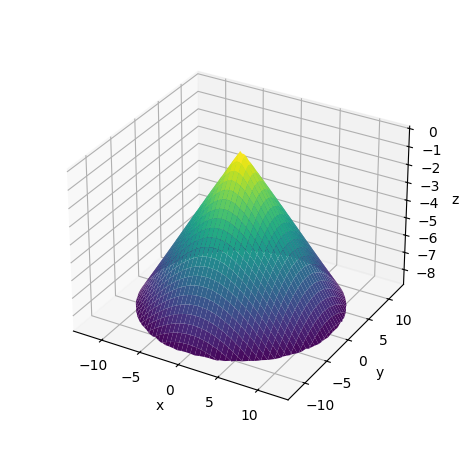
Let’s see what the surface looks like by plotting it in 3D.
[4]:
x = np.linspace(-12, 12, 256)
x, y = np.meshgrid(x, x)
z = new_geo.sag(x, y)  # <-- get the z values for the surface from "sag" method

# filter out points outside the aperture
r2 = x**2 + y**2
z[r2 > 12**2] = np.nan

fig = plt.figure()
ax = fig.add_subplot(111, projection="3d")
ax.plot_surface(x, y, z, cmap="viridis")
ax.set_xlabel("x")
ax.set_ylabel("y")
ax.set_zlabel("z")
ax.set_box_aspect(None, zoom=0.85)  # to avoid cutting off z label
plt.tight_layout()
plt.show()
Surface Definition
Now that we’ve defined our geometry, we also need to define the other components of our surface. In particular, we need to define the materials on each side of the surface. As this surface is the first surface of our system, the “pre-surface” material will simply be air and the “post-surface” material we will define as Schott SF2. There are other properties of the surface that can be added, such as coatings, scattering behavior, or physical apertures, but we will ignore these.
[5]:
material_pre = IdealMaterial(n=1.0)  # air
material_post = Material(name="SF2", reference="hikari")
We now have all components needed to generate our surface. We will also specify this surface as the aperture stop.
We omit the interaction model input, which results in the surface defaulting to a refractive component. See the API or docs on how to specify other interaction types.
[6]:
new_surface = Surface(
    geometry=new_geo,
    previous_surface=None,
    material_post=material_post,
    is_stop=True,
)
[7]:
lens = optic.Optic()

# add surfaces
lens.surfaces.add(index=0, radius=np.inf, thickness=np.inf)
lens.surfaces.add(
    index=1,
    new_surface=new_surface,
    thickness=15,
)  # <-- new surface added here
lens.surfaces.add(index=2, radius=-100, thickness=50)
lens.surfaces.add(index=3)

# add aperture
lens.set_aperture(aperture_type="EPD", value=25)

# add field
lens.fields.set_type(field_type="angle")
lens.fields.add(y=0)

# add wavelength
lens.wavelengths.add(value=0.55, is_primary=True)
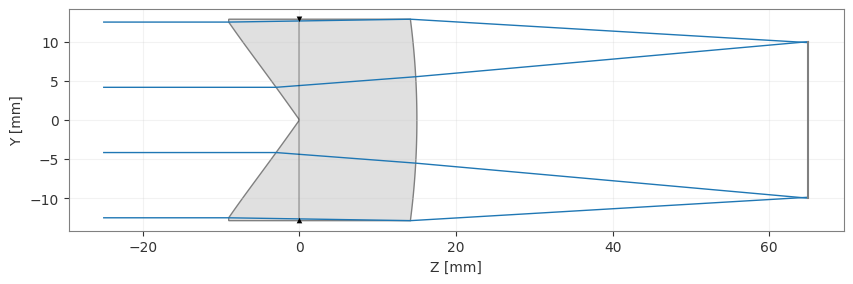
[8]:
_ = lens.draw(num_rays=10, xlim=(-30, 75))
[9]:
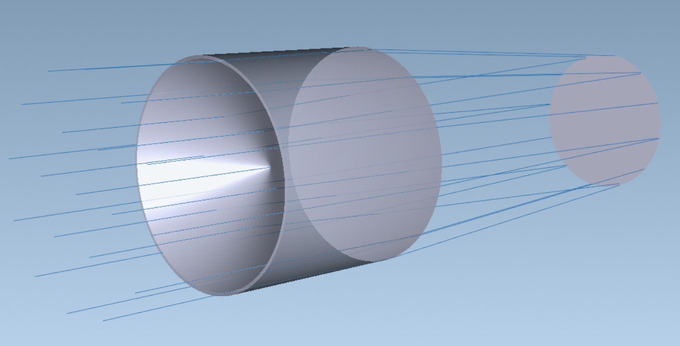
lens.draw3D(distribution="uniform", num_rays=8) # opens a new window, but we show a photo of the output below
`
While this lens form may not be particularly useful or practical, the concepts shown here can be used to define a surface with any desired geometry.
Conclusions
We demonstrated how a custom surface type can be created and added to an optical system in Optiland.
Creating a new surface type entails defining a new geometry, in which the surface sag equation and surface normal equation are defined.
Once the custom surface is defined, it can be used like any other surface in Optiland.