
Tutorial 10a: Non-Sequential & Illumination#
Most Optiland tutorials use the sequential engine: light passes through a known, ordered list of surfaces toward a single image plane. That is the right tool for imaging design. But many problems are not imaging problems:
How uniform is the light an LED throws onto a screen?
Where does stray light and how many ghost reflections land on my sensor?
How efficient is a non-imaging concentrator or light pipe?
For these, Optiland ships a differentiable non-sequential (NSQ) engine. Rays propagate freely through a 3-D scene and interact with surfaces in any order — reflecting, refracting, and scattering wherever they go. This tutorial is a short on-ramp; the NSQ gallery is the deep dive.
Two engines, two jobs. NSQ runs forward on NumPy (fast, 1e7+ rays — the production illumination/stray-light path, used here) and differentiably on PyTorch (optimize a scene with
loss.backward()). See gallery notebook 11.
1. A small illumination scene#
An NSQ model is an NSQScene holding sources, components, and detectors, each placed with a CoordinateSystem. Units: wavelengths in µm, positions in mm, angles in radians (config fields ending in _deg are degrees).
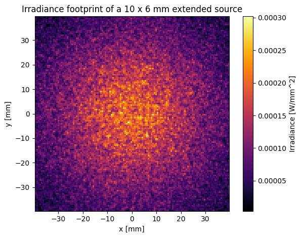
Here we throw a rectangular, LED-like ExtendedSource onto a screen and read the irradiance footprint — no lens, just free propagation.
[1]:
import matplotlib.pyplot as plt

from optiland.coordinate_system import CoordinateSystem
from optiland.nonsequential import (
    NSQScene, Spectrum, ExtendedSourceConfig, IrradianceDetectorConfig,
)

scene = NSQScene()
spec = Spectrum.monochromatic(0.55)          # 550 nm (wavelengths are in micrometres)

# A 10 x 6 mm extended (LED-like) emitter into a 60-degree half-angle cone
scene.add_source(
    'LED', CoordinateSystem(z=0),
    ExtendedSourceConfig(spectrum=spec, total_flux=1.0,
                         width=10, height=6, half_angle_deg=60),
)
# A screen 40 mm downstream
scene.add_detector(
    'screen', CoordinateSystem(z=40),
    IrradianceDetectorConfig(width=80, height=80, num_pixels_x=128, num_pixels_y=128),
)

# Forward trace on the NumPy engine
result = scene.trace(num_rays=200_000, max_depth=16, seed=0)

screen = result.detectors['screen']
print(f"Flux launched  : {result.total_flux_in:.3f} W")
print(f"Flux on screen : {screen.total_flux:.3f} W  ({screen.num_rays_hit:,} rays)")

fig = screen.plot(cmap='inferno')
plt.title('Irradiance footprint of a 10 x 6 mm extended source')
plt.tight_layout()
plt.show()
Flux launched  : 1.000 W
Flux on screen : 0.666 W  (133,123 rays)
2. Reading detectors#
scene.trace(...) returns a SimulationResult. Its .detectors dict is keyed by the names you assigned; each value is a result object — here an IrradianceMap with .irradiance (a W/mm² pixel array), .total_flux, .num_rays_hit, and a .plot() helper. The SimulationResult itself also carries flux-conservation bookkeeping (total_flux_in, total_flux_detected, num_rays_escaped, num_rays_depth_killed, …).
Other detectors record different physics: FarFieldDetector (angular intensity), SpectralDetector (per-wavelength), and RayDatabaseDetector (every ray’s full phase-space record). They are covered in gallery notebook 04.
3. Already have a lens? Convert it for stray-light analysis#
The fastest on-ramp for existing Optiland users: take any sequential Optic and convert it to an NSQScene in one line. sequential_to_nonsequential maps singlets to Lens, cemented doublets to Doublet, and the image surface to an IrradianceDetector. Because NSQ models Fresnel reflections at every uncoated interface, the trace reveals ghost reflections that the sequential engine never shows (the sequential engine always transmits 100% at an uncoated surface).
Conversion is never perfectly lossless — a sequential system doesn’t carry everything NSQ needs (explicit apertures, mirror reflectance, coatings), so the converter has to default, estimate, or drop what’s missing. Every such decision is recorded on the returned scene as scene.conversion_report, a structured record you can inspect instead of having to parse warning text — read it before trusting a converted trace.
[2]:
import warnings

from optiland.samples.objectives import CookeTriplet
from optiland.nonsequential import sequential_to_nonsequential

optic = CookeTriplet()

with warnings.catch_warnings():
    # The converter also raises a plain warning for the same information;
    # scene.conversion_report below is the structured version of it, so we
    # silence the warning and inspect the report instead.
    warnings.simplefilter('ignore')
    ghost_scene = sequential_to_nonsequential(optic)

print(ghost_scene.conversion_report.summary())

# max_depth high enough to let rays bounce between surfaces and form ghosts
result = ghost_scene.trace(num_rays=100_000, max_depth=32, seed=0)

# Ghost flux is faint by construction (a few percent of the beam, several
# bounces deep), so always check result.report() before trusting the numbers:
# a converted, multi-bounce scene like this one is exactly where an
# undersampled detector or truncated-depth flux would otherwise go unnoticed.
print(result.report())

det_name = list(result.detectors)[0]         # converter names the image detector
img = result.detectors[det_name]

fig = img.plot(cmap='hot')
plt.title('Cooke triplet image plane — direct image + Fresnel ghosts')
plt.tight_layout()
plt.show()

print(f"\nImage-plane flux: {img.total_flux:.4f} W from {img.num_rays_hit:,} rays")
Bare Fresnel, no sequential coating found (6): L1.front, L1.back, L3.front, L3.back, L5.front, L5.back
Apertures estimated (not explicitly set) (6): L1.front, L1.back, L3.front, L3.back, L5.front, L5.back
NSQ trace diagnostics:
  depth_truncated_flux_fraction: 0.0000%
  rr_killed_flux_fraction:       0.0000%
  flux_conservation_error:       0.0000%
  unreached_geometry:            none
  medium_stack_underflows:       0
  split_budget_saturated:        False
  detectors:
    D1: 54478 hits, 0.21 mean hits/pixel [undersampled]
Warnings:
  - Detector 'D1' is undersampled: 0.2 mean hits/pixel (< 10), shot noise dominates the map; ~192,476,963 rays would bring it to ~5% relative error.
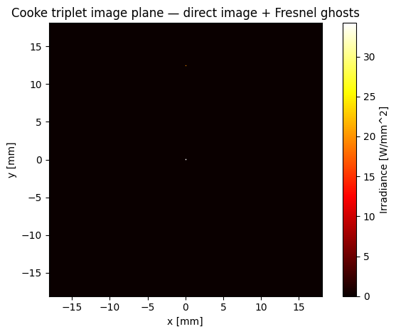
Image-plane flux: 1.6329 W from 54,478 rays
Where to go next#
This was the teaser. The NSQ gallery is the full deep dive:
01–05 — getting started, ray sources, optical components, detectors & results, surface scattering (BSDFs).
06–10 — diagnostics, multi-source illumination, stray-light/ghost analysis, reflective systems, advanced topics.
11 — Differentiable optimization. Switch to the PyTorch backend and reshape a detector’s irradiance by optimizing a lens radius via
loss.backward().
NSQ is pre-release (never shipped in a tagged Optiland version), so its API may still change. For the current capability envelope and known limitations (notably zero visibility gradients), see the canonical NSQ Limitations & Roadmap page.