
Tutorial 1a: Optiland for Beginners#
Last verified against Optiland v0.6.1.
This tutorial describes the basics of Optiland. In particular, the following topics are covered:
Basic lens entry
Material definition and selection
Aperture, field and wavelength selection
Checking a system for common mistakes
Drawing a lens in 2D and 3D
A complete lens, first#
Below is a full, working optical system: a singlet with a 25 mm entrance pupil, one on-axis field, and one wavelength. Run it and you get a ray-traced layout. Everything after this cell explains what each line does — but the whole program is already here, and it is not long.
[1]:
import numpy as np

from optiland import optic
[3]:
singlet = optic.Optic()

# define surfaces
singlet.surfaces.add(index=0, radius=np.inf, thickness=np.inf)
singlet.surfaces.add(index=1, radius=20, thickness=7, is_stop=True, material="N-SF11")
singlet.surfaces.add(index=2, radius=np.inf, thickness=18)
singlet.surfaces.add(index=3)

# define aperture
singlet.set_aperture(aperture_type="EPD", value=25)

# define fields
singlet.fields.set_type(field_type="angle")
singlet.fields.add(y=0)

# define wavelengths
singlet.wavelengths.add(value=0.5, is_primary=True)

# draw it
singlet.draw(num_rays=10)
[3]:
(<Figure size 1000x400 with 1 Axes>, <Axes: xlabel='Z [mm]', ylabel='Y [mm]'>)
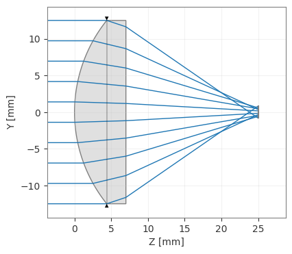
Note:Thedraw()method returns the matplotlib figure and axes.When running Optiland in a script, you must explicitly callplt.show()orfig.show()to display the plot.
In Jupyter notebooks, figures are displayed automatically.
That is the entire program. The rest of this tutorial takes it apart line by line.
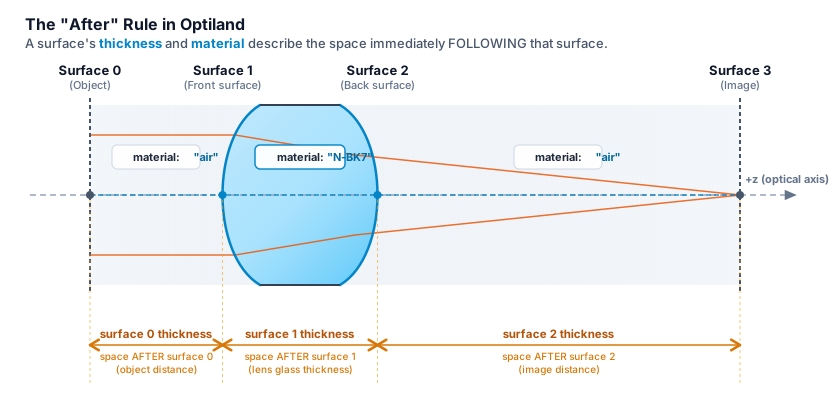
One convention to internalize before you read further: a surface’s
thicknessandmaterialdescribe the space that follows it, not the surface itself. Sosurfaces.add(index=1, thickness=7, material="N-SF11")means 7 mm of N-SF11 glass between surface 1 and surface 2.
The full set of conventions — sign conventions, units, the object/image surface rule, and stop vs. aperture vs. pupil — lives on the Conventions page. It is worth the five minutes.
Defining a lens, in detail:#
Create the optic:#
In Optiland, lenses are instances of the “Optic” class. The process for defining a lens starts with creating an empty “Optic” object as follows:
[4]:
lens = optic.Optic()
Add the object surface:#
We now want to populate the lens object with surfaces. Let’s first add the object surface, which will be at infinity and will have a radius of infinity, i.e. it is a plane. We add the surface by calling the “add_surface” method. We must specify the index as 0 to indicate this is the first surface.
[5]:
lens.surfaces.add(index=0, radius=np.inf, thickness=np.inf)
Add a lens:#
Let’s now add a singlet lens:
Material: N-SF11
Thickness: 7 mm
Radius side 1: 20 mm
Radius side 2: infinity
Stop surface: 1
Optiland defines lenses one surface at a time, so each side of the lens is a separate surface — indices 1 and 2 here, following the object plane at index 0.
Because thickness and material describe the space after a surface (the “after” rule above), surface 1 carries thickness=7, material="N-SF11" — the glass — and surface 2 carries thickness=18, the air gap to the image plane. Surface 2 needs no material: air is the default. See Conventions for the sign conventions and units that go with this.
[6]:
lens.surfaces.add(index=1, thickness=7, radius=20, is_stop=True, material="N-SF11")
lens.surfaces.add(index=2, radius=np.inf, thickness=18)
Add image plane:#
Lastly, let’s add the image plane. By default, the radius is infinity, so we can exclude it. We also can omit thickness, as there are no surfaces beyond the image. We need only to define the index, which is 3.
[7]:
lens.surfaces.add(index=3)
Define aperture:#
Now, we can define the aperture of the system. Let’s choose entrance pupil diameter (EPD) as the aperture type with a value of 25 mm.
The options for aperture type are:
‘EPD’ - entrance pupil diameter
‘imageFNO’ - image-space F-number
‘objectNA’ - object-space numerical aperture
‘float_by_stop_size’ - the aperture size floats with the size of the stop diameter, which is defined by the
valueargument.
[8]:
lens.set_aperture(aperture_type="EPD", value=25)
Define fields:#
Let’s add the fields of the lens. We’ll keep it simple and add a single field of type “angle” with a value of 0.
The options for field types are:
‘angle’ - the angle of the field in object space
‘object_height’ - the height of the object
‘paraxial_image_height’ - the image height of a paraxial chief ray
‘real_image_height’ - the image height of a real chief ray
[9]:
lens.fields.set_type(field_type="angle")
lens.fields.add(y=0)
Define wavelengths:#
Lastly, let’s define the wavelengths of the system. We define a single wavelength at 0.5 µm. Similar to fields, wavelengths can be assigned a weight to emphasize specific spectral regions.
[10]:
lens.wavelengths.add(value=0.5, is_primary=True)
Sanity-check the lens:#
Before viewing or tracing rays through the lens, it is good practice to run check_system. It inspects the Optic for the mistakes newcomers hit most often (a missing wavelength, an undefined aperture, a stop that was never marked, …) and reports each one with a runnable fix. report.ok is True once there are no errors left.
[11]:
from optiland.diagnostics import check_system

report = check_system(lens)
report
[11]:
DiagnosticReport: no issues found.
View the lens:#
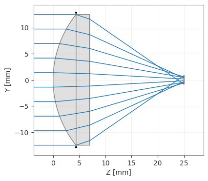
Let’s view the lens in 2D. We can do this by calling the draw method.
Note that you can also pass a projection argument, allowing you to plot in the "YZ" plane (default), "XZ" plane, or "XY" plane.
The 2D visualization is now interactive! You can hover over surfaces, lenses, and ray bundles to get more information. You can also customize the look and feel of the plots using themes. See the gallery for an example of how to use themes.
[12]:
lens.draw(num_rays=10)
[12]:
(<Figure size 1000x400 with 1 Axes>, <Axes: xlabel='Z [mm]', ylabel='Y [mm]'>)
[13]:
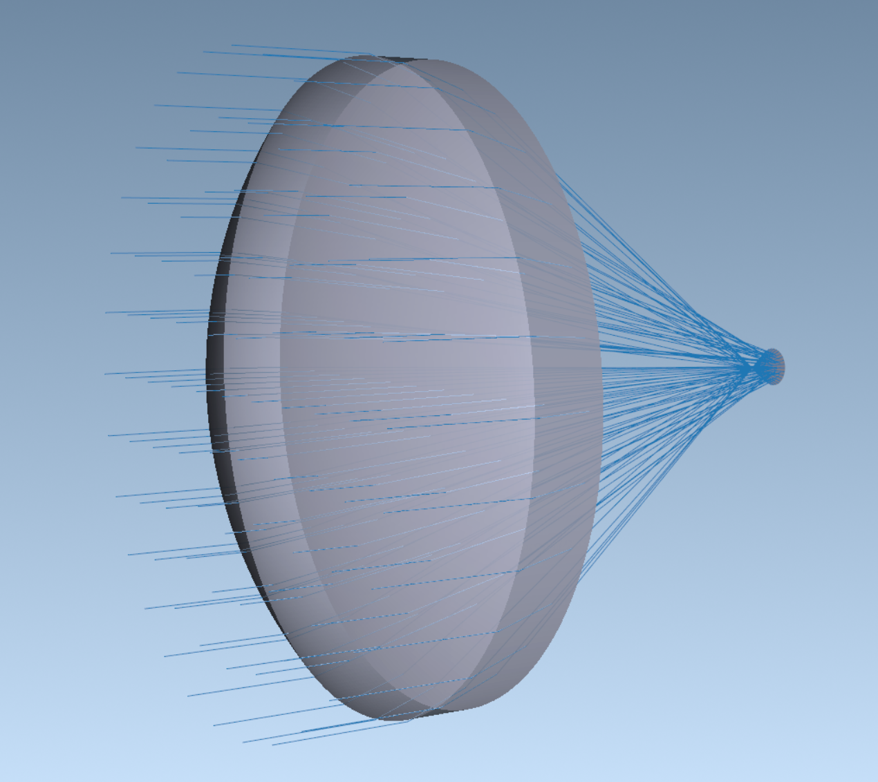
lens.draw3D()
The 3D view opens in a separate VTK window rather than inline, so here is what it looks like:
Where to go next#
You can now build an optical system from scratch, define its aperture, fields and wavelengths, check it for common mistakes, and view it in 2D and 3D. That is enough to enter any sequential system Optiland supports.
Next steps, in order of usefulness:
Tutorial 1b — Lens Properties and Prescription — read the first-order properties (EFL, f/#, pupils) back out of a system.
Tutorial 1e — Design a Doublet End to End — one design carried from requirements through analysis, optimization and tolerancing.
Conventions — the model behind every tutorial, in one page.
How do I …? — a task-shaped index: find your question, get the notebook that answers it.