Zernike Decomposition
Decompose complex wavefronts into orthogonal polynomial modes.
Introduction
This tutorial shows how to decompose the pupil using various Zernike types. Namely, we use "standard", "fringe", and "Noll" Zernike indices.
Core concepts used
Step-by-step build
Import wavefront module and sample eyepiece
import matplotlib.pyplot as plt

from optiland import wavefront
from optiland.samples.eyepieces import EyepieceErfleInstantiate and draw the Erfle eyepiece
lens = EyepieceErfle()
lens.draw()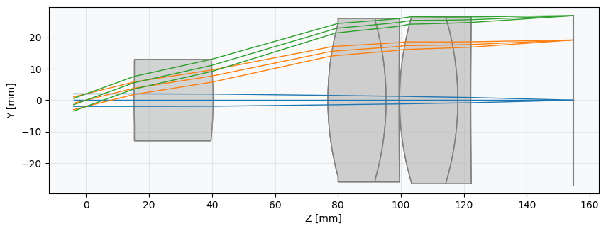
View the on-axis OPD map
First, we'll view the wavefront.
opd = wavefront.OPD(lens, field=(0, 0), wavelength=0.55)
opd.view(projection="2d", num_points=512)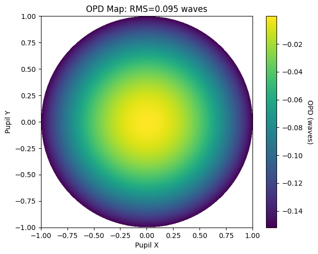
Fit standard Zernike polynomials to the wavefront
We'll then find the Zernike coefficients of the wavefront.
zernike_standard = wavefront.ZernikeOPD(
 lens,
 field=(0, 0),
 wavelength=0.55,
 zernike_type="standard",
 num_terms=37,
)View the Zernike-reconstructed OPD map
Let's view the Zernike fit and compare it to the nominal OPD map.
zernike_standard.view(projection="2d", num_points=512)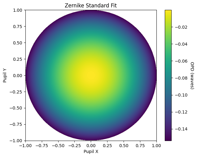
Plot the standard Zernike coefficient bar chart
Qualitatively, we can see the Zernike fit well-represents the OPD map.
Let's see what the actual coefficients look like:
plt.bar(range(1, 38), zernike_standard.coeffs)
plt.axhline(color="k", linewidth=1, linestyle="--")
plt.xlabel("Zernike Term #")
plt.ylabel("Zernike Standard Coefficient")
plt.show()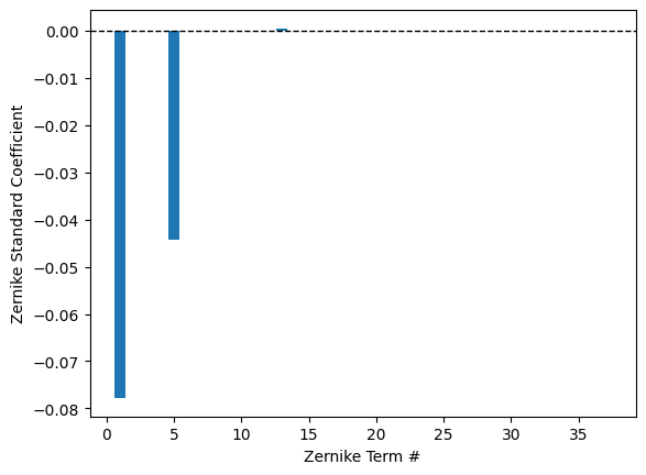
Decompose full-field wavefront using fringe Zernike indices
Let's decompose the wavefront using Zernike fringe indices and Zernike Noll indices. We'll use the field point at (0, 1).
zernike_fringe = wavefront.ZernikeOPD(
 lens,
 field=(0, 1),
 wavelength=0.55,
 zernike_type="fringe",
 num_terms=37,
)

plt.bar(range(1, 38), zernike_fringe.coeffs, color="C1")
plt.axhline(color="k", linewidth=1, linestyle="--")
plt.xlabel("Zernike Term #")
plt.ylabel("Zernike Fringe Coefficient")
plt.show()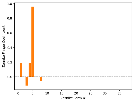
Decompose full-field wavefront using Noll Zernike indices
zernike_noll = wavefront.ZernikeOPD(
 lens,
 field=(0, 1),
 wavelength=0.55,
 zernike_type="noll",
 num_terms=37,
)

plt.bar(range(1, 38), zernike_noll.coeffs, color="C2")
plt.axhline(color="k", linewidth=1, linestyle="--")
plt.xlabel("Zernike Term #")
plt.ylabel("Zernike Noll Coefficient")
plt.show()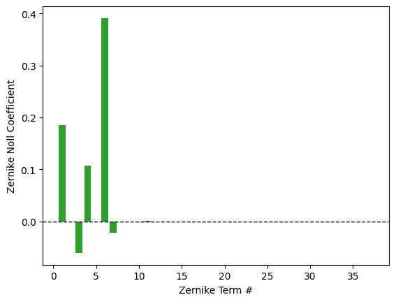
Print Noll Zernike coefficients numerically
Or, if we just want to read off the coefficients, we can print them. Let's only use 9 terms in this case:
zernike = wavefront.ZernikeOPD(lens, (0, 1), 0.55, zernike_type="noll", num_terms=9)

for k in range(len(zernike.coeffs)):
 print(f"Z{k + 1}: {zernike.coeffs[k]:.8f}")
Show full code listing
import matplotlib.pyplot as plt

from optiland import wavefront
from optiland.samples.eyepieces import EyepieceErfle

lens = EyepieceErfle()
lens.draw()

opd = wavefront.OPD(lens, field=(0, 0), wavelength=0.55)
opd.view(projection="2d", num_points=512)

zernike_standard = wavefront.ZernikeOPD(
  lens,
  field=(0, 0),
  wavelength=0.55,
  zernike_type="standard",
  num_terms=37,
)

zernike_standard.view(projection="2d", num_points=512)

plt.bar(range(1, 38), zernike_standard.coeffs)
plt.axhline(color="k", linewidth=1, linestyle="--")
plt.xlabel("Zernike Term #")
plt.ylabel("Zernike Standard Coefficient")
plt.show()

zernike_fringe = wavefront.ZernikeOPD(
  lens,
  field=(0, 1),
  wavelength=0.55,
  zernike_type="fringe",
  num_terms=37,
)

plt.bar(range(1, 38), zernike_fringe.coeffs, color="C1")
plt.axhline(color="k", linewidth=1, linestyle="--")
plt.xlabel("Zernike Term #")
plt.ylabel("Zernike Fringe Coefficient")
plt.show()

zernike_noll = wavefront.ZernikeOPD(
  lens,
  field=(0, 1),
  wavelength=0.55,
  zernike_type="noll",
  num_terms=37,
)

plt.bar(range(1, 38), zernike_noll.coeffs, color="C2")
plt.axhline(color="k", linewidth=1, linestyle="--")
plt.xlabel("Zernike Term #")
plt.ylabel("Zernike Noll Coefficient")
plt.show()

zernike = wavefront.ZernikeOPD(lens, (0, 1), 0.55, zernike_type="noll", num_terms=9)

for k in range(len(zernike.coeffs)):
  print(f"Z{k + 1}: {zernike.coeffs[k]:.8f}")
Conclusions
- The
wavefront.ZernikeOPDclass fits an arbitrary number of Zernike polynomial terms to a sampled OPD map, providing a compact, analytically useful representation of complex wavefront errors. - Standard, fringe, and Noll indexing conventions are all supported via the
zernike_typeparameter, making it straightforward to match the convention used by external tools such as interferometers or adaptive-optics software. - Visualising the reconstructed OPD map alongside the raw map confirms that 37 terms capture the dominant wavefront structure of the Erfle eyepiece with high fidelity.
- Bar charts of the coefficient vectors immediately reveal which polynomial modes — such as defocus, primary astigmatism, or higher-order coma — carry the largest contribution at a given field point.
- Printing coefficients numerically with a reduced term count (e.g. 9 terms) offers a concise, machine-readable summary suitable for tolerance budgeting or further numerical processing.
Next tutorials
Original notebook: Tutorial_4c_Zernike_Decomposition.ipynb on GitHub · ReadTheDocs