PSF and MTF Calculation
Convert wavefront data into Point Spread Functions and MTF curves.
Introduction
This tutorial shows how to calculate the point spread function (PSF) and modulation transfer function (MTF) of a lens.
Core concepts used
Step-by-step build
Import PSF and MTF modules
from optiland import mtf, psf
from optiland.samples.objectives import CookeTripletInstantiate and draw the Cooke Triplet
lens = CookeTriplet()
lens.draw()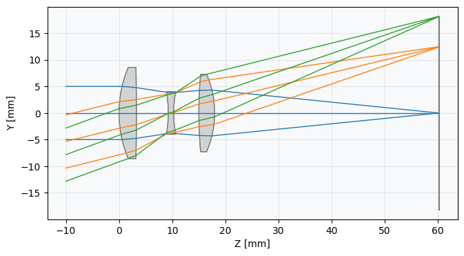
Compute and view the on-axis FFT PSF in 3D
We first compute the PSF using the FFT-based approach. We demonstrate various ways to generate and plot the PSF.
lens_psf = psf.FFTPSF(lens, field=(0, 0), wavelength=0.55)
lens_psf.view(projection="3d", num_points=256)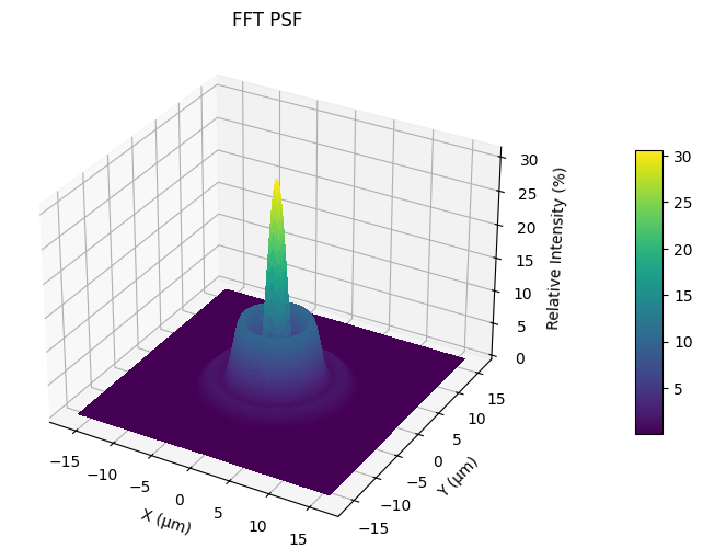
Calculate the Strehl ratio
print(f"Strehl Ratio: {lens_psf.strehl_ratio():.3f}")View the FFT PSF at 0.7 field height
lens_psf = psf.FFTPSF(lens, field=(0, 0.7), wavelength=0.55)
lens_psf.view(num_points=512)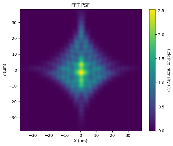
View the FFT PSF at full field in 2D
lens_psf = psf.FFTPSF(lens, field=(0, 1.0), wavelength=0.55)
lens_psf.view(projection="2d", num_points=256)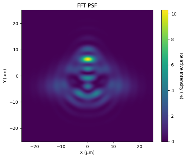
Compute the Huygens PSF at full field
We can also generate the PSF using direct Huygens-Fresnel integration. This is referred to as the "Huygens PSF".
lens_huygens_psf = psf.HuygensPSF(lens, field=(0, 1.0), wavelength=0.55)
lens_huygens_psf.view(projection="2d", num_points=256)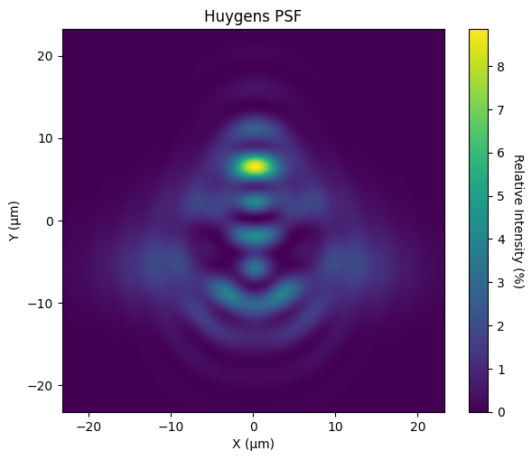
Plot the geometric MTF
Now, we generate the geometric MTF, which uses only ray intersection locations on the image plane and ignores diffraction. The geometric MTF is a reasonable approximation when the lens is far from the diffraction limit.
As is standard, the geometric MTF is scaled based on the diffraction-limited MTF curve. This assures that the geometric MTF cannot show performance better than the diffraction limit.
geo_mtf = mtf.GeometricMTF(lens)
geo_mtf.view()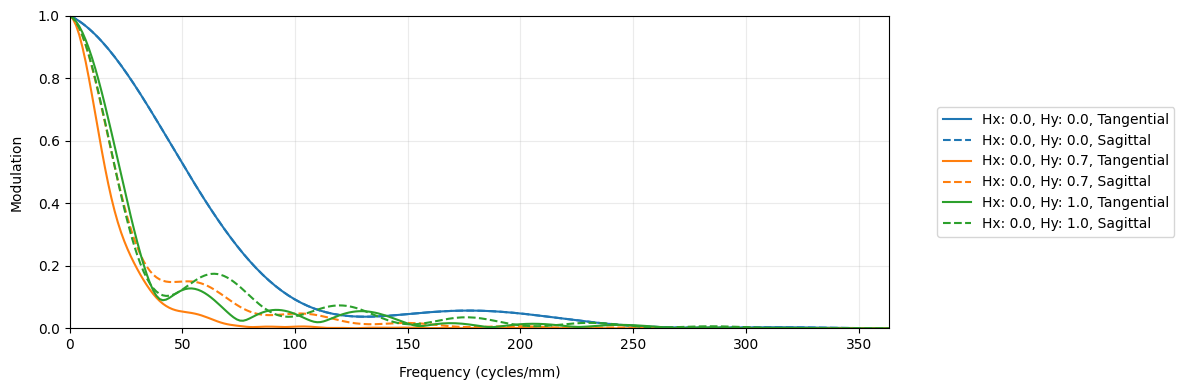
Plot the diffraction-based FFT MTF
Finally, we show the standard FFT-based MTF.
lens_mtf = mtf.FFTMTF(lens)
lens_mtf.view()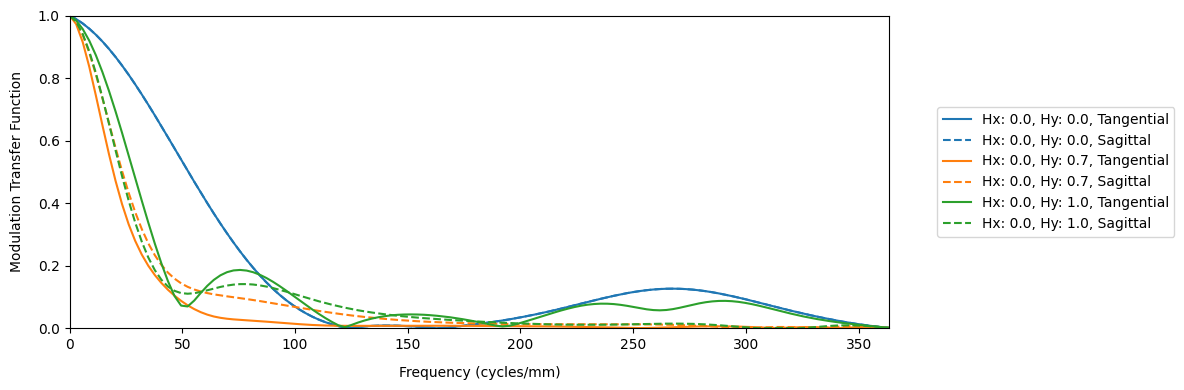
Show full code listing
from optiland import mtf, psf
from optiland.samples.objectives import CookeTriplet

lens = CookeTriplet()
lens.draw()

lens_psf = psf.FFTPSF(lens, field=(0, 0), wavelength=0.55)
lens_psf.view(projection="3d", num_points=256)

print(f"Strehl Ratio: {lens_psf.strehl_ratio():.3f}")

lens_psf = psf.FFTPSF(lens, field=(0, 0.7), wavelength=0.55)
lens_psf.view(num_points=512)

lens_psf = psf.FFTPSF(lens, field=(0, 1.0), wavelength=0.55)
lens_psf.view(projection="2d", num_points=256)

lens_huygens_psf = psf.HuygensPSF(lens, field=(0, 1.0), wavelength=0.55)
lens_huygens_psf.view(projection="2d", num_points=256)

geo_mtf = mtf.GeometricMTF(lens)
geo_mtf.view()

lens_mtf = mtf.FFTMTF(lens)
lens_mtf.view()
Conclusions
- The FFT PSF (
psf.FFTPSF) efficiently converts the pupil function into an irradiance distribution at the image plane and supports both 2D and 3D projection modes for visual inspection at any field position. - The Strehl ratio — retrieved via
strehl_ratio()— provides a single, normalized metric that captures overall wavefront quality relative to a perfect diffraction-limited system. - The Huygens PSF (
psf.HuygensPSF) offers an alternative integration-based calculation that can be more robust for highly aberrated systems where the FFT approximation breaks down. - The geometric MTF (
mtf.GeometricMTF) gives a fast, ray-based estimate of spatial-frequency contrast that is automatically capped by the diffraction-limited envelope, making it useful as a rapid design-stage check. - The diffraction-based FFT MTF (
mtf.FFTMTF) yields the most physically accurate modulation transfer function by propagating the full complex pupil, enabling rigorous performance evaluation across all field positions.
Next tutorials
Original notebook: Tutorial_4b_PSF_%26_MTF_Calculation.ipynb on GitHub · ReadTheDocs