OPD Calculations
Understand the phase of the light as it propagates through your lens.
Introduction
This tutorial demonstrates how to compute the optical path difference in the exit pupil and the various ways to plot it.
Core concepts used
Step-by-step build
Import libraries and load the Erfle eyepiece
Import the wavefront module and instantiate the built-in Erfle eyepiece, then draw the system layout for reference.
from optiland import wavefront
from optiland.samples.eyepieces import EyepieceErfle

lens = EyepieceErfle()
lens.draw()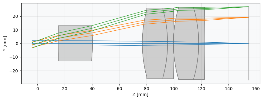
Compute and view the OPD fan across all fields
Compute the OPD fans for each field point and wavelength. The OPD fan shows the wavefront error across the pupil — analogous to a ray fan, but for phase.
opd_fan = wavefront.OPDFan(lens)
opd_fan.view()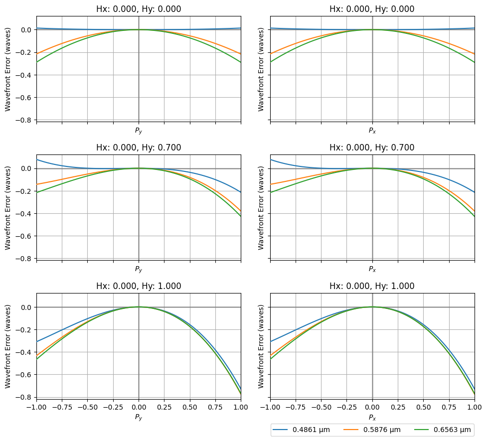
View the on-axis wavefront error map in 2D
Compute a high-resolution wavefront map for the on-axis field and render it as a 2D color map to inspect the aberration structure.
opd = wavefront.OPD(lens, field=(0, 0), wavelength=0.5876)
opd.view(projection="2d", num_points=512)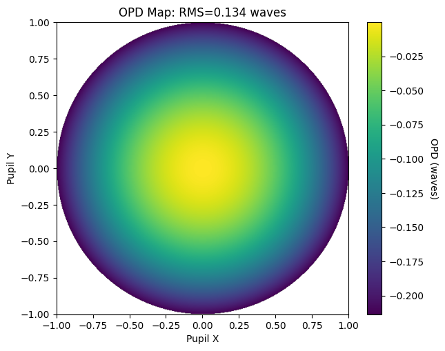
View the 70% field wavefront error map in 2D
Repeat the same 2D wavefront map at 70% field height to see how off-axis aberrations begin to dominate.
opd = wavefront.OPD(lens, field=(0, 0.7), wavelength=0.5876)
opd.view(projection="2d", num_points=512)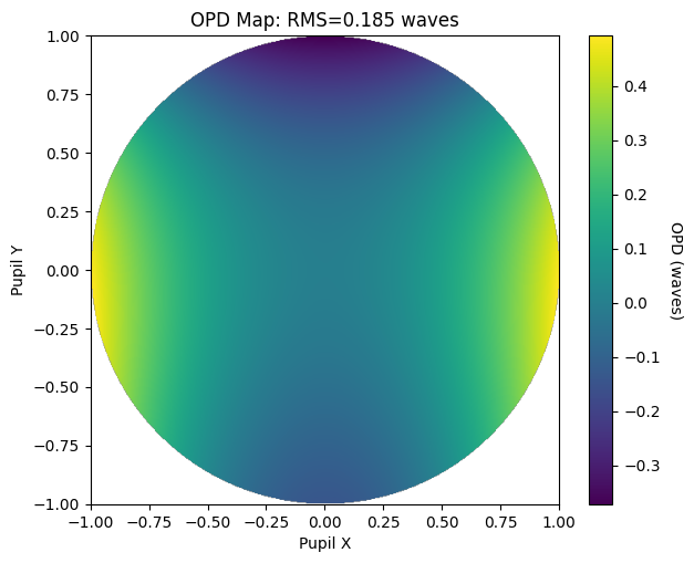
Render the full-field wavefront error as a 3D surface
Switch to the "3d" projection at full field to visualize the wavefront topography — coma ridges and astigmatism saddles become immediately apparent.
opd = wavefront.OPD(lens, field=(0, 1.0), wavelength=0.5876)
opd.view(projection="3d", num_points=512)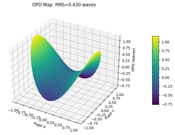
Show full code listing
from optiland import wavefront
from optiland.samples.eyepieces import EyepieceErfle

lens = EyepieceErfle()
lens.draw()

opd_fan = wavefront.OPDFan(lens)
opd_fan.view()

opd = wavefront.OPD(lens, field=(0, 0), wavelength=0.5876)
opd.view(projection="2d", num_points=512)

opd = wavefront.OPD(lens, field=(0, 0.7), wavelength=0.5876)
opd.view(projection="2d", num_points=512)

opd = wavefront.OPD(lens, field=(0, 1.0), wavelength=0.5876)
opd.view(projection="3d", num_points=512)
Conclusions
This tutorial covered the two main OPD tools in Optiland:
OPDFangives a compact, multi-field view of the wavefront error across the pupil — useful for quickly spotting which aberrations dominate at each field point.OPDcomputes a full high-resolution wavefront map for a single field and wavelength, with a choice of 2D color map or 3D surface projections.- Comparing on-axis (pure spherical) with 70% and full-field maps clearly reveals how coma and astigmatism grow with field angle.
- The
rms()method can convert anyOPDmap to a single merit-function number for use in optimization or tolerance budgets.
Next tutorials
Original notebook: Tutorial_4a_Optical_Path_Difference_Calculation.ipynb on GitHub · ReadTheDocs