Chromatic Aberrations
Analyze longitudinal and lateral color effects across the visible spectrum.
Introduction
This tutorial demonstrates how to assess chromatic aberrations in Optiland. We will first investigate a singlet with poor color correction, and then a well-corrected achromatic doublet.
Core concepts used
Step-by-step build
Import numpy, analysis, and optic
import numpy as np

from optiland import analysis, opticDefine the high-dispersion N-SF6 Singlet class
Let's define a simple singlet using a material with high dispersion:
class Singlet(optic.Optic):
 """Simple Singlet"""

 def __init__(self):
     super().__init__()

     # add surfaces
     self.add_surface(index=0, radius=np.inf, thickness=np.inf)
     self.add_surface(
         index=1,
         thickness=0.5,
         radius=32.2526,
         is_stop=True,
         material="N-SF6",
     )
     self.add_surface(index=2, thickness=19.8532, radius=-31.9756)
     self.add_surface(index=3)

     # add aperture
     self.set_aperture(aperture_type="EPD", value=3.4)

     # add field
     self.set_field_type(field_type="angle")
     self.add_field(y=0.0)

     # add wavelength
     self.add_wavelength(value=0.48613270)
     self.add_wavelength(value=0.58756180, is_primary=True)
self.add_wavelength(value=0.65627250)Draw the singlet with multiple wavelengths
singlet = Singlet()
singlet.draw(
 wavelengths=[0.48613270, 0.587561806, 0.65627250],
 figsize=(16, 4),
 num_rays=3,
)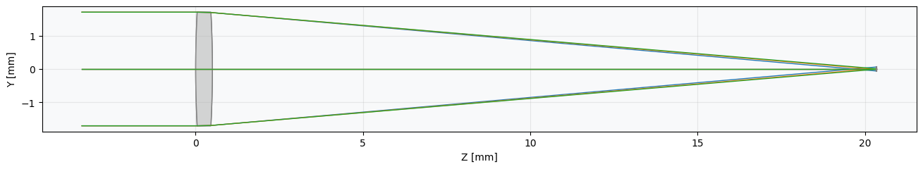
Compute first-order longitudinal axial color for the singlet
As can be seen in the visualization, the wavelengths of light focus at different points on the optical axis (zooming in can also help to see this more clearly). To quantify this, let's compute the first-order longitudinal axial color:
print(f"First-order Longitudinal Color: {np.sum(singlet.aberrations.LchC()):.3f}")Plot the ray fan aberrations for the singlet
This can also be seen in ray aberration plots. The slope of the tranverse errors at the and locations vary with wavelength. This indicates that the defocus differs as a function of wavelength.
fan = analysis.RayFan(singlet)
fan.view()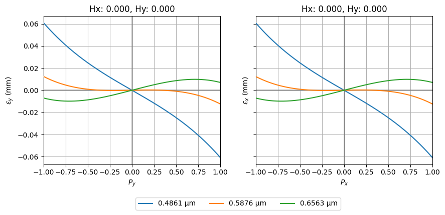
Define the achromatic N-BAK1/SF2 Doublet class
Now, let's define an achromatic doublet, which improves the chromatic aberration performance in comparison to our simple singlet:
class Doublet(optic.Optic):
 """Achromatic Doublet

 Milton Laikin, Lens Design, 4th ed., CRC Press, 2007, p. 45
 """

 def __init__(self):
     super().__init__()

     # add surfaces
     self.add_surface(index=0, radius=np.inf, thickness=np.inf)
     self.add_surface(
         index=1,
         radius=12.38401,
         thickness=0.4340,
         is_stop=True,
         material="N-BAK1",
     )
     self.add_surface(
         index=2,
         radius=-7.94140,
         thickness=0.3210,
         material=("SF2", "schott"),
     )
     self.add_surface(index=3, radius=-48.44396, thickness=19.6059)
     self.add_surface(index=4)

     # add aperture
     self.set_aperture(aperture_type="EPD", value=3.4)

     # add field
     self.set_field_type(field_type="angle")
     self.add_field(y=0)

     # add wavelength
     self.add_wavelength(value=0.48613270)
     self.add_wavelength(value=0.58756180, is_primary=True)
self.add_wavelength(value=0.65627250)Draw the doublet with multiple wavelengths
doublet = Doublet()
doublet.draw(
 wavelengths=[0.48613270, 0.587561806, 0.65627250],
 figsize=(16, 4),
 num_rays=3,
)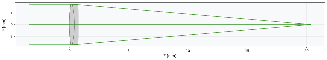
Compute first-order longitudinal axial color for the doublet
We can already see that the various wavelengths appear to focus at a similar location. Let's confirm that the longitudinal chromatic aberration has indeed been reduced by computing this directly and generating the tranverse ray aberrations plots.
print(f"First-order Longitudinal Color: {np.sum(doublet.aberrations.LchC()):.3f}")Plot the ray fan aberrations for the doublet
This value was -0.789 for the singlet and is now -0.015 for the doublet, which is a significant improvement. Now let's look at the tranverse ray aberration plots:
fan = analysis.RayFan(doublet)
fan.view()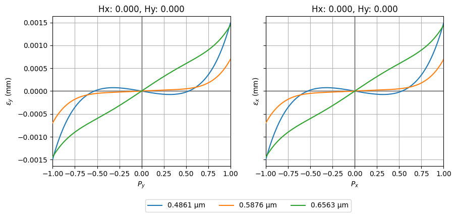
Show full code listing
import numpy as np

from optiland import analysis, optic

class Singlet(optic.Optic):
  """Simple Singlet"""

  def __init__(self):
      super().__init__()

      # add surfaces
      self.add_surface(index=0, radius=np.inf, thickness=np.inf)
      self.add_surface(
          index=1,
          thickness=0.5,
          radius=32.2526,
          is_stop=True,
          material="N-SF6",
      )
      self.add_surface(index=2, thickness=19.8532, radius=-31.9756)
      self.add_surface(index=3)

      # add aperture
      self.set_aperture(aperture_type="EPD", value=3.4)

      # add field
      self.set_field_type(field_type="angle")
      self.add_field(y=0.0)

      # add wavelength
      self.add_wavelength(value=0.48613270)
      self.add_wavelength(value=0.58756180, is_primary=True)
      self.add_wavelength(value=0.65627250)

singlet = Singlet()
singlet.draw(
  wavelengths=[0.48613270, 0.587561806, 0.65627250],
  figsize=(16, 4),
  num_rays=3,
)

print(f"First-order Longitudinal Color: {np.sum(singlet.aberrations.LchC()):.3f}")

fan = analysis.RayFan(singlet)
fan.view()

class Doublet(optic.Optic):
  """Achromatic Doublet

  Milton Laikin, Lens Design, 4th ed., CRC Press, 2007, p. 45
  """

  def __init__(self):
      super().__init__()

      # add surfaces
      self.add_surface(index=0, radius=np.inf, thickness=np.inf)
      self.add_surface(
          index=1,
          radius=12.38401,
          thickness=0.4340,
          is_stop=True,
          material="N-BAK1",
      )
      self.add_surface(
          index=2,
          radius=-7.94140,
          thickness=0.3210,
          material=("SF2", "schott"),
      )
      self.add_surface(index=3, radius=-48.44396, thickness=19.6059)
      self.add_surface(index=4)

      # add aperture
      self.set_aperture(aperture_type="EPD", value=3.4)

      # add field
      self.set_field_type(field_type="angle")
      self.add_field(y=0)

      # add wavelength
      self.add_wavelength(value=0.48613270)
      self.add_wavelength(value=0.58756180, is_primary=True)
      self.add_wavelength(value=0.65627250)

doublet = Doublet()
doublet.draw(
  wavelengths=[0.48613270, 0.587561806, 0.65627250],
  figsize=(16, 4),
  num_rays=3,
)

print(f"First-order Longitudinal Color: {np.sum(doublet.aberrations.LchC()):.3f}")

fan = analysis.RayFan(doublet)
fan.view()
Conclusions
Note that the y-axis scale of this plot is significantly smaller than that of the singlet. We can confirm that chromatic aberrations have been significantly reduced.
Next tutorials
Original notebook: Tutorial_3c_Chromatic_Aberrations.ipynb on GitHub · ReadTheDocs