Material Database
Access thousands of glasses from Schott, Ohara, and other major vendors.
Introduction
This tutorial introduces the main material abstractions available in Optiland, from simple idealized media to real catalog data pulled through the refractiveindex.info integration. The goal is to show when each material class is appropriate and how to evaluate refractive index programmatically as a function of wavelength.
You will work through fixed-index materials, Abbe-number-based glass models, and database-backed materials such as glasses, organics, liquids, crystals, and gases.
Core concepts used
n and extinction coefficient k across all wavelengths.Step-by-step build
Import material and plotting utilities
import matplotlib.pyplot as plt
import numpy as np

from optiland.materials import AbbeMaterial, AbbeMaterialE, IdealMaterial, MaterialCreate a fixed-index ideal material
The IdealMaterial class represents a material with a fixed refractive index and extinction coefficient. This is useful for simulations that require simple, constant parameters.
ideal_material = IdealMaterial(n=1.5, k=0)

wavelengths = [0.48, 0.55, 0.65]

for wavelength in wavelengths:
 print(f"Refractive Index at {wavelength} µm: {ideal_material.n(wavelength)}")
 print(
     f"Extinction Coefficient at {wavelength} µm: {ideal_material.k(wavelength)}",
     end="\n\n",
)Compare the available Abbe material models
The AbbeMaterial class generates a model optical glass material in the visible spectrum. The material is defined by its refractive index at a reference wavelength and its Abbe number. Optiland supports two distinct definitions:
-
Standard d-line ():
- Reference (): Helium d-line at 587.56 nm.
- Abbe Number (): Calculated using Hydrogen F (486.1 nm) and C (656.3 nm) lines.
- Models: "buchdahl" (Recommended) and "polynomial" (Legacy).
-
e-line ():
- Reference (): Mercury e-line at 546.07 nm.
- Abbe Number (): Calculated using Cadmium F' (480.0 nm) and C' (643.8 nm) lines.
- Model:
AbbeMaterialEclass.
The extinction coefficient is set to zero for these models but can be overwritten manually.
# Create instances of the different Abbe models

# 1. Buchdahl Model (d-line) - The new recommended default
# Input: Index at 587.56 nm, Abbe number Vd (using F/C lines)
abbe_buchdahl = AbbeMaterial(n=1.5, abbe=65.0, model="buchdahl")

# 2. Legacy Polynomial Model (d-line)
# Input: Index at 587.56 nm, Abbe number Vd (using F/C lines)
abbe_poly = AbbeMaterial(n=1.5, abbe=65.0, model="polynomial")

# 3. AbbeMaterialE (e-line)
# Input: Index at 546.07 nm, Abbe number Ve (using F'/C' lines)
# Note: Ve is typically slightly different from Vd for the same physical glass.
abbe_e = AbbeMaterialE(n=1.5, abbe=65.0)

# Define wavelength range for plotting
wavelengths = np.linspace(0.4, 0.75, 500)

# Calculate refractive indices
n_buchdahl = abbe_buchdahl.n(wavelengths)
n_poly = abbe_poly.n(wavelengths)
n_e = abbe_e.n(wavelengths)

# Plot the results
plt.figure(figsize=(10, 6))
plt.plot(wavelengths, n_buchdahl, label='Buchdahl (d-line: 587nm, F/C)', linestyle='-')
plt.plot(wavelengths, n_poly, label='Polynomial (Legacy)', linestyle='--')
plt.plot(wavelengths, n_e, label='Buchdahl (e-line: 546nm, F\'/C\')', linestyle='-.')

plt.xlabel("Wavelength (µm)")
plt.ylabel("Refractive Index")
plt.title("Comparison of Abbe Material Models (n=1.5, V=65.0)")
plt.legend()
plt.grid(alpha=0.25)
plt.show()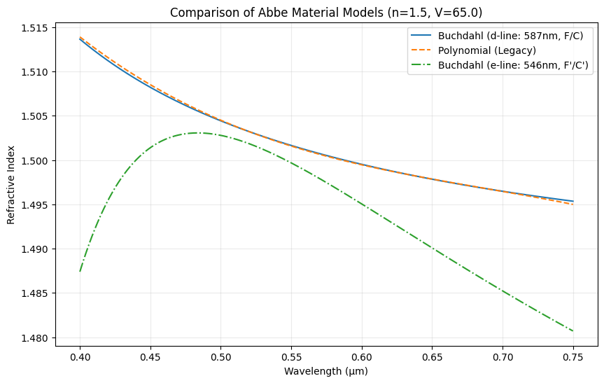
Load a catalog glass from the database
The Material class connects to refractiveindex.info to access real-world material data. It uses string matching to find the closest match for a given material name.
Example 1: A common glass type
glass = Material("N-SF5")

n_sf5 = glass.n(wavelengths)

plt.plot(wavelengths, n_sf5, "C1")
plt.xlabel("Wavelength (µm)")
plt.ylabel("Refractive Index")
plt.title("Refractive Index of N-SF5 vs. Wavelength")
plt.grid(alpha=0.25)
plt.show()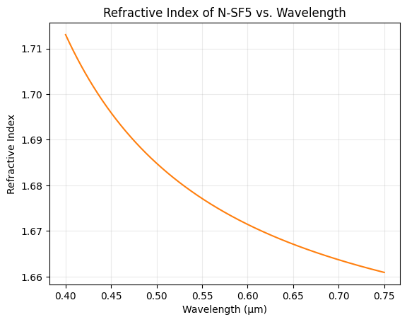
Narrow the match with a vendor reference
Note that you may also pass a reference name to the material, which narrows down the material selection if there are multiple matches for the given material name. The reference can include e.g., the glass manufacturer, the author name, year of publication, etc.
glass = Material("N-SF5", reference="Schott")Query an organic material
DNA = Material("DNA")

wavelength = 0.26

# call `.item()` to get the value as a scalar
print(f"Refractive Index of DNA at {wavelength} µm: {DNA.n(wavelength).item():.5f}")Query additional real materials
silver_chloride = Material("AgCl")
toluene = Material("toluene")

wavelength = 0.55

n_agcl = silver_chloride.n(wavelength).item()
print(f"Refractive Index of AgCl at {wavelength} µm: {n_agcl:.5f}")
n_toluene = toluene.n(wavelength).item()
print(f"Refractive Index of toluene at {wavelength} µm: {n_toluene:.5f}")Example 4 Gases (helium)
he = Material("He")

wavelength = 0.612

print(f"Refractive Index of He at {wavelength} µm: {he.n(wavelength).item():.7f}")
Show full code listing
import matplotlib.pyplot as plt
import numpy as np

from optiland.materials import AbbeMaterial, AbbeMaterialE, IdealMaterial, Material

ideal_material = IdealMaterial(n=1.5, k=0)

wavelengths = [0.48, 0.55, 0.65]

for wavelength in wavelengths:
  print(f"Refractive Index at {wavelength} µm: {ideal_material.n(wavelength)}")
  print(
      f"Extinction Coefficient at {wavelength} µm: {ideal_material.k(wavelength)}",
      end="\n\n",
  )

# Create instances of the different Abbe models

# 1. Buchdahl Model (d-line) - The new recommended default
# Input: Index at 587.56 nm, Abbe number Vd (using F/C lines)
abbe_buchdahl = AbbeMaterial(n=1.5, abbe=65.0, model="buchdahl")

# 2. Legacy Polynomial Model (d-line)
# Input: Index at 587.56 nm, Abbe number Vd (using F/C lines)
abbe_poly = AbbeMaterial(n=1.5, abbe=65.0, model="polynomial")

# 3. AbbeMaterialE (e-line)
# Input: Index at 546.07 nm, Abbe number Ve (using F'/C' lines)
# Note: Ve is typically slightly different from Vd for the same physical glass.
abbe_e = AbbeMaterialE(n=1.5, abbe=65.0)

# Define wavelength range for plotting
wavelengths = np.linspace(0.4, 0.75, 500)

# Calculate refractive indices
n_buchdahl = abbe_buchdahl.n(wavelengths)
n_poly = abbe_poly.n(wavelengths)
n_e = abbe_e.n(wavelengths)

# Plot the results
plt.figure(figsize=(10, 6))
plt.plot(wavelengths, n_buchdahl, label='Buchdahl (d-line: 587nm, F/C)', linestyle='-')
plt.plot(wavelengths, n_poly, label='Polynomial (Legacy)', linestyle='--')
plt.plot(wavelengths, n_e, label='Buchdahl (e-line: 546nm, F\'/C\')', linestyle='-.')

plt.xlabel("Wavelength (µm)")
plt.ylabel("Refractive Index")
plt.title("Comparison of Abbe Material Models (n=1.5, V=65.0)")
plt.legend()
plt.grid(alpha=0.25)
plt.show()

glass = Material("N-SF5")

n_sf5 = glass.n(wavelengths)

plt.plot(wavelengths, n_sf5, "C1")
plt.xlabel("Wavelength (µm)")
plt.ylabel("Refractive Index")
plt.title("Refractive Index of N-SF5 vs. Wavelength")
plt.grid(alpha=0.25)
plt.show()

glass = Material("N-SF5", reference="Schott")

DNA = Material("DNA")

wavelength = 0.26

# call `.item()` to get the value as a scalar
print(f"Refractive Index of DNA at {wavelength} µm: {DNA.n(wavelength).item():.5f}")

silver_chloride = Material("AgCl")
toluene = Material("toluene")

wavelength = 0.55

n_agcl = silver_chloride.n(wavelength).item()
print(f"Refractive Index of AgCl at {wavelength} µm: {n_agcl:.5f}")
n_toluene = toluene.n(wavelength).item()
print(f"Refractive Index of toluene at {wavelength} µm: {n_toluene:.5f}")

he = Material("He")

wavelength = 0.612

print(f"Refractive Index of He at {wavelength} µm: {he.n(wavelength).item():.7f}")
Conclusions
This tutorial showcased the key features of the Optiland material database. By leveraging IdealMaterial, AbbeMaterial, and Material, users can simulate a wide variety of optical systems with realistic material properties.
Next tutorials
Original notebook: Tutorial_1d_Material_Database.ipynb on GitHub · ReadTheDocs