Singlet Lens
Build and trace a simple single-element lens in Optiland — learning the core syntax for surface definition, aperture, fields, and wavelengths.
Introduction
This tutorial walks through the construction of a simple singlet lens in Optiland. Instead of starting from a long finished script, it first shows the complete system once and then rebuilds it piece by piece so you can see how surfaces, aperture, fields, and wavelengths fit together.
By the end, you will know the minimal workflow for defining and visualizing a sequential optical system from scratch.
Core concepts used
Step-by-step build
Preview the complete singlet script
This shows the full code to generate a singlet lens. In the next section, we will go into each part of this code in more detail.
import numpy as np

from optiland import optic

singlet = optic.Optic()

# define surfaces
singlet.add_surface(index=0, radius=np.inf, thickness=np.inf)
singlet.add_surface(index=1, radius=20, thickness=7, is_stop=True, material="N-SF11")
singlet.add_surface(index=2, radius=np.inf, thickness=18)
singlet.add_surface(index=3)

# define aperture
singlet.set_aperture(aperture_type="EPD", value=25)

# define fields
singlet.set_field_type(field_type="angle")
singlet.add_field(y=0)

# define wavelengths
singlet.add_wavelength(value=0.5, is_primary=True)

# view in 3D - Note this opens a new window, but we add a photo below to
# show the visualization
singlet.draw3D()Preview the initial 2D layout
# view in 2D
singlet.draw(num_rays=10)
Start the detailed lens definition
Note:
Thedraw()method returns the matplotlib figure and axes.
When running Optiland in a script, you must explicitly callplt.show()orfig.show()to display the plot.
In Jupyter notebooks, figures are displayed automatically.
Create the optic:
In Optiland, lenses are instances of the "Optic" class. The process for defining a lens starts with creating an empty "Optic" object as follows:
lens = optic.Optic()Add the object surface
We now want to populate the lens object with surfaces. Let's first add the object surface, which will be at infinity and will have a radius of infinity, i.e. it is a plane. We add the surface by calling the "add_surface" method. We must specify the index as 0 to indicate this is the first surface.
lens.add_surface(index=0, radius=np.inf, thickness=np.inf)Add the singlet element
Let's now add a singlet lens. The lens will be defined as follows:
- Material: N-SF11
- Thickness: 7 mm
- Radius side 1: 20 mm
- Radius side 2: infinity
- Stop surface: 1
Optiland defines lenses one surface at a time, so we define each side of the lens separately. The material always corresponds to the material after interaction with a surface (refraction or reflection). Likewise, the thickness corresponds to the thickness after the surface and it is positive for surfaces to the right. This also implies that we must define the distance from the second surface to the next surface, which we'll define as 18 mm.
Note that we specify the indices of the two surfaces as 1 and 2, after we already specified the object plane with index 0. Also note that Optiland uses millimeters by default.
lens.add_surface(index=1, thickness=7, radius=20, is_stop=True, material="N-SF11")
lens.add_surface(index=2, radius=np.inf, thickness=18)Add the image plane
Lastly, let's add the image plane. By default, the radius is infinity, so we can exclude it. We also can omit thickness, as there are no surfaces beyond the image. We need only to define the index, which is 3.
lens.add_surface(index=3)Set the system aperture
Now, we can define the aperture of the system. Let's choose entrance pupil diameter (EPD) as the aperture type with a value of 25 mm.
The options for aperture type are:
-
'EPD' - entrance pupil diameter
-
'imageFNO' - image-space F-number
-
'objectNA' - object-space numerical aperture
-
'float_by_stop_size' - the aperture size floats with the size of the stop diameter, which is defined by the
valueargument.pythonlens.set_aperture(aperture_type="EPD", value=25)
Add the on-axis field
Let's add the fields of the lens. We'll keep it simple and add a single field of type "angle" with a value of 0.
The options for field types are:
-
'angle' - the angle of the field in object space
-
'object_height' - the height of the object
-
'paraxial_image_height' - the image height of a paraxial chief ray
-
'real_image_height' - the image height of a real chief ray
pythonlens.set_field_type(field_type="angle") lens.add_field(y=0)
Define the design wavelength
Lastly, let's define the wavelengths of the system. We define a single wavelength at 0.5 µm.
lens.add_wavelength(value=0.5, is_primary=True)Draw the finished lens
Let's view the lens in 2D. We can do this by calling the draw method.
Note that you can also pass a projection argument, allowing you to plot in the "YZ" plane (default), "XZ" plane, or "XY" plane.
The 2D visualization is now interactive! You can hover over surfaces, lenses, and ray bundles to get more information. You can also customize the look and feel of the plots using themes. See the gallery for an example of how to use themes.
lens.draw(num_rays=10)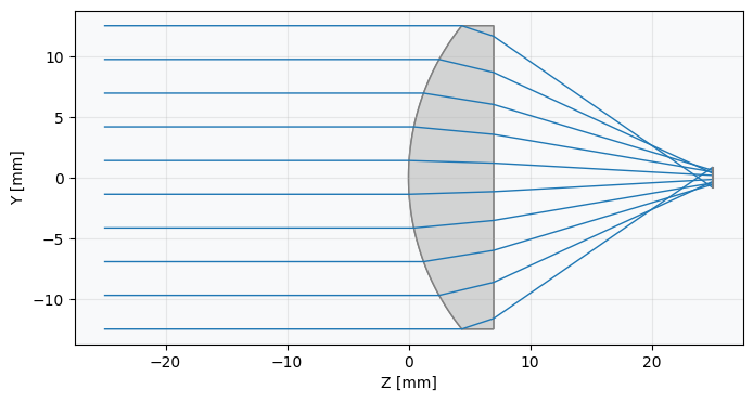
Render the 3D interactive visualization
Finally, we view the lens in 3D using the "draw3D" function. Note that this opens a new window.
lens.draw3D()Show full code listing
import numpy as np
from optiland import optic
singlet = optic.Optic()
# define surfaces
singlet.add_surface(index=0, radius=np.inf, thickness=np.inf)
singlet.add_surface(index=1, radius=20, thickness=7, is_stop=True, material="N-SF11")
singlet.add_surface(index=2, radius=np.inf, thickness=18)
singlet.add_surface(index=3)
# define aperture
singlet.set_aperture(aperture_type="EPD", value=25)
# define fields
singlet.set_field_type(field_type="angle")
singlet.add_field(y=0)
# define wavelengths
singlet.add_wavelength(value=0.5, is_primary=True)
# view in 3D - Note this opens a new window, but we add a photo below to
# show the visualization
singlet.draw3D()
# view in 2D
singlet.draw(num_rays=10)
lens = optic.Optic()
lens.add_surface(index=0, radius=np.inf, thickness=np.inf)
lens.add_surface(index=1, thickness=7, radius=20, is_stop=True, material="N-SF11")
lens.add_surface(index=2, radius=np.inf, thickness=18)
lens.add_surface(index=3)
lens.set_aperture(aperture_type="EPD", value=25)
lens.set_field_type(field_type="angle")
lens.add_field(y=0)
lens.add_wavelength(value=0.5, is_primary=True)
lens.draw(num_rays=10)
lens.draw3D()Conclusions
You have built your first optical system in Optiland. Along the way you learned:
- How to create an
Opticcontainer and populate it surface by surface usingadd_surface(). - How to control the aperture (
set_aperture()), field points (add_field()), and wavelengths (add_wavelength()). - How material assignment and thickness conventions work — material is defined after a surface, and thickness is the distance to the next surface.
- How to visualize the system in 2D with
draw()and in 3D withdraw3D().
This minimal workflow is the foundation for every optical design in Optiland, from a simple singlet to a complex multi-element system.
Next tutorials
Original notebook: Tutorial_1a_Optiland_for_Beginners.ipynb on GitHub · ReadTheDocs