Aberrations
Common Aberration Analyses
Bridge the gap between ray patterns and classical aberration theory.
IntermediateAberrationsNumPy backend12 min read
Introduction
This tutorial demonstrates the various aberration plots and analyses that can be performed in Optiland. Namely, we cover:
- Spot diagrams
- Ray fans
- Y-Ybar plots
- Distortion / Grid distortion plots
- Field curvature plots
Core concepts used
analysis.RayFan(lens)
Plots transverse ray aberrations as a function of pupil position. The "DNA" of an optical system's performance.
analysis.FieldCurvature(lens)
Visualizes the Petzval surface and the separation between sagittal and tangential focal planes.
analysis.Distortion(lens)
Quantifies the percentage deviation of image height from the ideal paraxial prediction ().
analysis.RmsSpotSizeVsField()
Plots how the aggregate blur changes as you move from the center to the corner of the image.
Step-by-step build
1
Import analysis modules
python
from optiland import analysis
from optiland.samples.objectives import CookeTriplet
2
Instantiate the Cooke Triplet and draw the lens layout
python
lens = CookeTriplet()
lens.draw()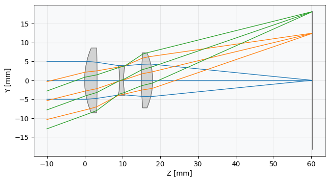
3
Plot the spot diagram
Spot Diagram
python
spot = analysis.SpotDiagram(lens)
spot.view()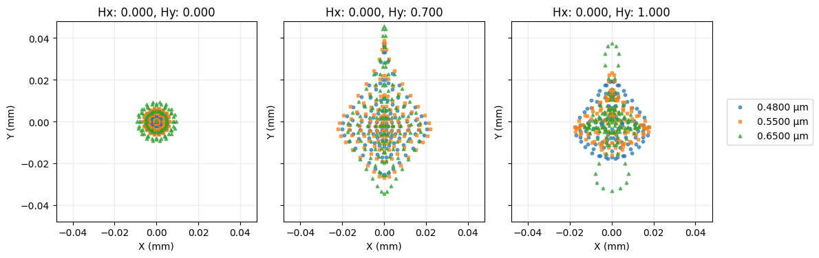
4
Extract field coordinates and compute spot radius statistics
python
fields = lens.fields.get_field_coords()
wavelengths = lens.wavelengths.get_wavelengths()

print("Geometric Spot Radius:")

geo_spot_radius = spot.geometric_spot_radius()
for i, field in enumerate(fields):
 for j, wavelength in enumerate(wavelengths):
     print(
         f"\tField {field}, Wavelength {wavelength:.3f} µm, "
         f"Radius: {geo_spot_radius[i][j]:.5f} mm",
     )

print("RMS Spot Radius:")

rms_spot_radius = spot.rms_spot_radius()
for i, field in enumerate(fields):
 for j, wavelength in enumerate(wavelengths):
     print(
         f"\tField {field}, Wavelength {wavelength:.3f} µm, "
         f"Radius: {rms_spot_radius[i][j]:.5f} mm",
     )
5
Plot the ray fan aberration diagram
Ray fans
python
fan = analysis.RayFan(lens)
fan.view()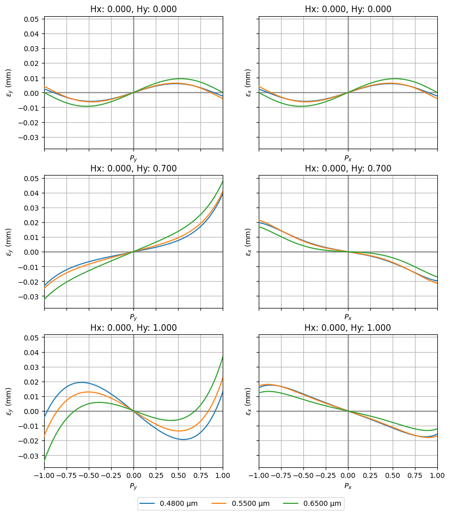
6
Plot the Y-Ybar diagram
Y-Ybar plot
python
yybar = analysis.YYbar(lens)
yybar.view()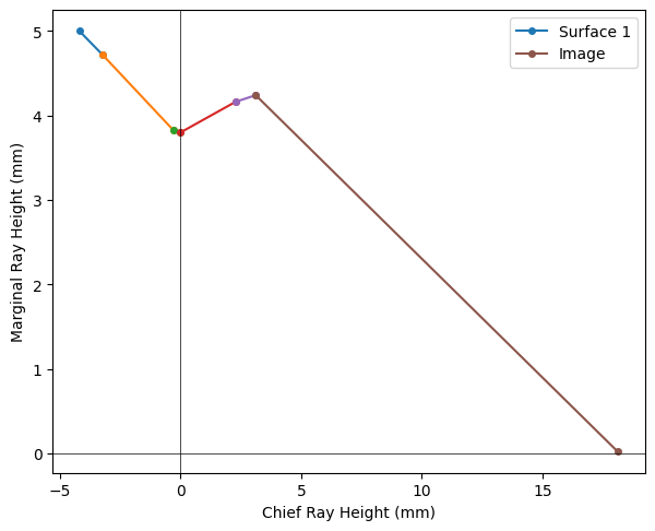
7
Plot the distortion map
Distortion
python
distortion = analysis.Distortion(lens)
distortion.view()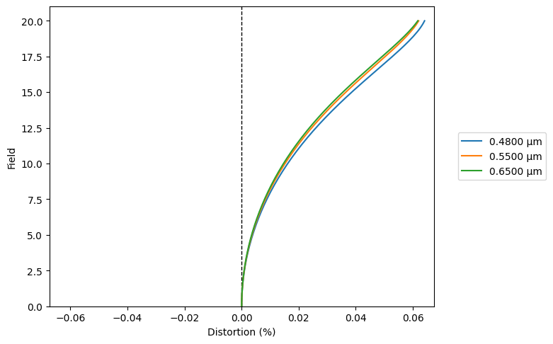
8
Plot the grid distortion map
Grid distortion
python
grid = analysis.GridDistortion(lens)
grid.view()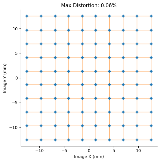
9
Plot the field curvature diagram
Field Curvature
python
field_curv = analysis.FieldCurvature(lens)
field_curv.view()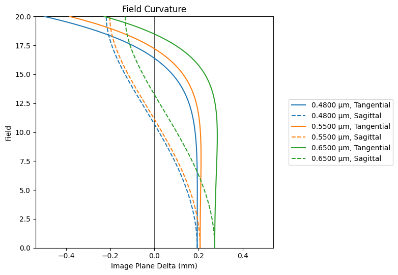
10
Plot RMS spot size versus field
RMS Spot Size vs. Field
python
rms_spot_vs_field = analysis.RmsSpotSizeVsField(lens)
rms_spot_vs_field.view()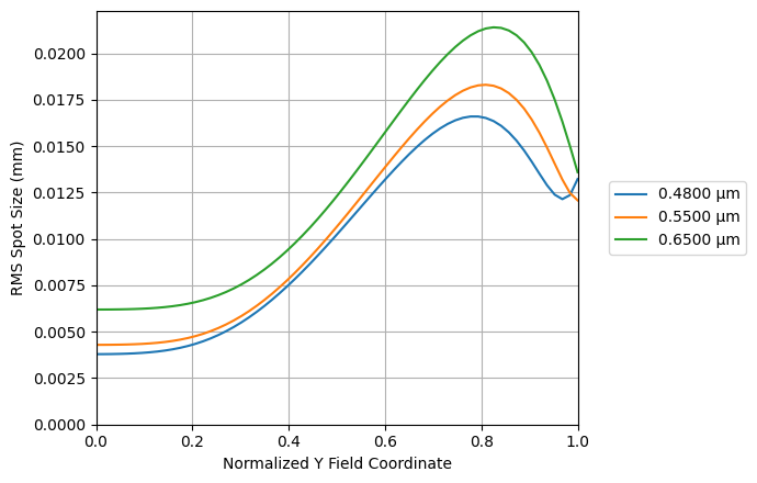
11
Plot RMS wavefront error versus field
RMS Wavefront Error vs. Field
python
rms_wavefront_error_vs_field = analysis.RmsWavefrontErrorVsField(lens)
rms_wavefront_error_vs_field.view()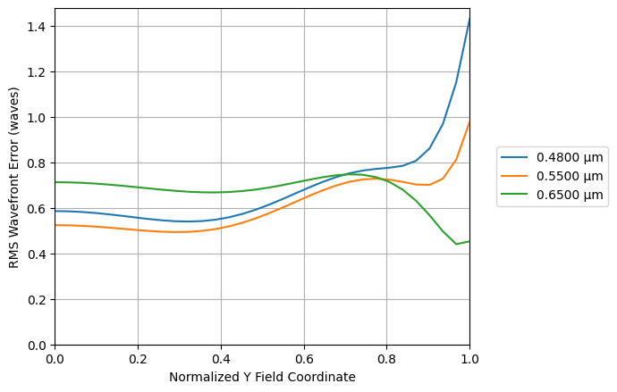
12
Plot the pupil aberration diagram
Pupil Aberration
- The pupil abberration is defined as the difference between the paraxial and real ray intersection point at the stop surface of the optic. This is specified as a percentage of the on-axis paraxial stop radius at the primary wavelength.
python
pupil_ab = analysis.PupilAberration(lens)
pupil_ab.view()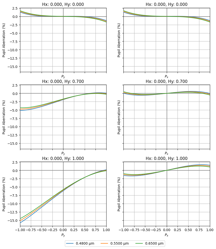
Show full code listing
python
from optiland import analysis
from optiland.samples.objectives import CookeTriplet

lens = CookeTriplet()
lens.draw()

spot = analysis.SpotDiagram(lens)
spot.view()

fields = lens.fields.get_field_coords()
wavelengths = lens.wavelengths.get_wavelengths()

print("Geometric Spot Radius:")

geo_spot_radius = spot.geometric_spot_radius()
for i, field in enumerate(fields):
  for j, wavelength in enumerate(wavelengths):
      print(
          f"\tField {field}, Wavelength {wavelength:.3f} µm, "
          f"Radius: {geo_spot_radius[i][j]:.5f} mm",
      )

print("RMS Spot Radius:")

rms_spot_radius = spot.rms_spot_radius()
for i, field in enumerate(fields):
  for j, wavelength in enumerate(wavelengths):
      print(
          f"\tField {field}, Wavelength {wavelength:.3f} µm, "
          f"Radius: {rms_spot_radius[i][j]:.5f} mm",
      )

fan = analysis.RayFan(lens)
fan.view()

yybar = analysis.YYbar(lens)
yybar.view()

distortion = analysis.Distortion(lens)
distortion.view()

grid = analysis.GridDistortion(lens)
grid.view()

field_curv = analysis.FieldCurvature(lens)
field_curv.view()

rms_spot_vs_field = analysis.RmsSpotSizeVsField(lens)
rms_spot_vs_field.view()

rms_wavefront_error_vs_field = analysis.RmsWavefrontErrorVsField(lens)
rms_wavefront_error_vs_field.view()

pupil_ab = analysis.PupilAberration(lens)
pupil_ab.view()
Conclusions
- Demonstrated eight analysis tools available in the
optiland.analysismodule on a Cooke Triplet:SpotDiagram,RayFan,YYbar,Distortion,GridDistortion,FieldCurvature,RmsSpotSizeVsField,RmsWavefrontErrorVsField, andPupilAberration. - Each analysis object follows the same two-step pattern — instantiate with the
lensobject, then call.view()— making the API consistent and easy to remember. - The YYbar diagram and distortion plots reveal field-dependent behavior, while the field curvature and pupil aberration plots highlight residual Seidel terms across the pupil.
- RMS spot size and RMS wavefront error vs. field provide a quick scalar summary of image quality, useful for comparing design iterations at a glance.
Next tutorials
Next1st & 3rd Order AberrationsDecompose performance into classical Seidel coefficients (S1 to S5).RelatedRaytracing AspheresSee how aspheric surfaces can be used to specifically target these analyzed aberrations.
Original notebook: Tutorial_3a_Common_Aberration_Analyses.ipynb on GitHub · ReadTheDocs