Ray Tracing

Raytracing Aspheres

Model components with non-spherical profiles for high-performance optics.

IntermediateRay TracingNumPy backend10 min read

Introduction

This tutorial shows how even aspheres can be modeled in Optiland. We will first assess a simple spherical lens, then compare it to an even asphere.

Core concepts used

surface_type='even_asphere'

Enables the standard polynomial asphere model in Optiland.

conic=k

Sets the conic constant (

k

). For example,

k=-1

creates a paraboloid, while

k=0

is a standard sphere.

coefficients=[a2, a4, ...]

A list of coefficients for the even terms of the radial expansion (

r^2, r^4, r^6, \dots

Step-by-step build

Import libraries

python

import numpy as np

from optiland import analysis, optic

Build and analyse the spherical singlet

Let's define a simple singlet:

python

spherical = optic.Optic()

# add surfaces
spherical.add_surface(index=0, radius=np.inf, thickness=np.inf)
spherical.add_surface(
 index=1,
 thickness=7,
 radius=20.0,
 is_stop=True,
 material="N-SF11",
)
spherical.add_surface(index=2, thickness=21.56201105)
spherical.add_surface(index=3)

# add aperture
spherical.set_aperture(aperture_type="EPD", value=20.0)

# add field
spherical.set_field_type(field_type="angle")
spherical.add_field(y=0)

# add wavelength
spherical.add_wavelength(value=0.587, is_primary=True)

spherical.update_paraxial()

spherical.draw(num_rays=10)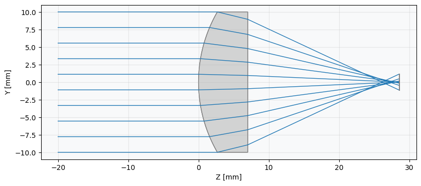

python

spot = analysis.SpotDiagram(spherical)
spot.view()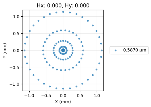

As we can see, this lens shows a significant amount of spherical aberration, as is typical for such a lens.

Build and analyse the aspheric singlet

Let's now define an asphere which has improved spherical aberration performance.

We define the "surface_type" attribute as "even_asphere" and we supply a list of coefficients of the aspheric terms. The aspheric surface sag equation is

z(r) = \frac{r^2}{R\left(1 + \sqrt{1 - (1 + \kappa)\frac{r^2}{R^2}}\right)} + \alpha_2 r^2 + \alpha_4 r^4 + \alpha_6 r^6 + \ldots

where $z$ is the sag, $R$ is the radius of curvature, $r$ is the radial distance from the optical axis, and $\alpha_2, \alpha_4, \alpha_6, \ldots$ are the coefficients of the asphere. The coefficient list provided to the surface is simply $[\alpha_2, \alpha_4, \alpha_6, \ldots]$ .

python

asphere = optic.Optic()

# add surfaces
asphere.add_surface(index=0, radius=np.inf, thickness=np.inf)
asphere.add_surface(
 index=1,
 thickness=7,
 radius=20.0,
 is_stop=True,
 material="N-SF11",
 surface_type="even_asphere",
 conic=0.0,
 coefficients=[
     -2.248851e-4,
     -4.690412e-6,
     -6.404376e-8,
 ],  # <-- coefficients for asphere
)
asphere.add_surface(index=2, thickness=21.56201105)
asphere.add_surface(index=3)

# add aperture
asphere.set_aperture(aperture_type="EPD", value=20.0)

# add field
asphere.set_field_type(field_type="angle")
asphere.add_field(y=0)

# add wavelength
asphere.add_wavelength(value=0.587, is_primary=True)

asphere.update_paraxial()

asphere.draw(num_rays=5)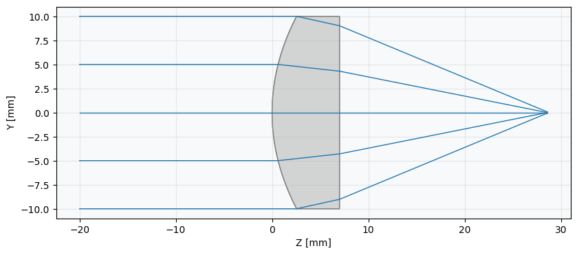

python

spot = analysis.SpotDiagram(asphere)
spot.view()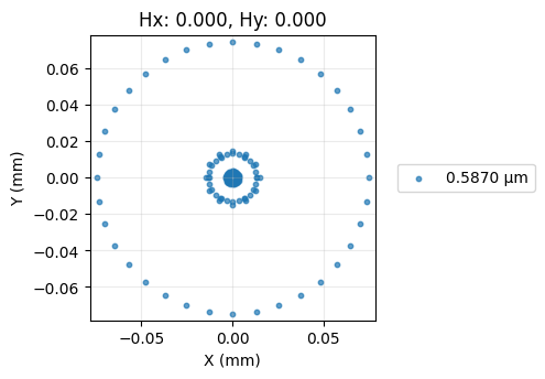

Show full code listing

python

import numpy as np

from optiland import analysis, optic

spherical = optic.Optic()

# add surfaces
spherical.add_surface(index=0, radius=np.inf, thickness=np.inf)
spherical.add_surface(
  index=1,
  thickness=7,
  radius=20.0,
  is_stop=True,
  material="N-SF11",
)
spherical.add_surface(index=2, thickness=21.56201105)
spherical.add_surface(index=3)

# add aperture
spherical.set_aperture(aperture_type="EPD", value=20.0)

# add field
spherical.set_field_type(field_type="angle")
spherical.add_field(y=0)

# add wavelength
spherical.add_wavelength(value=0.587, is_primary=True)

spherical.update_paraxial()

spherical.draw(num_rays=10)

spot = analysis.SpotDiagram(spherical)
spot.view()

asphere = optic.Optic()

# add surfaces
asphere.add_surface(index=0, radius=np.inf, thickness=np.inf)
asphere.add_surface(
  index=1,
  thickness=7,
  radius=20.0,
  is_stop=True,
  material="N-SF11",
  surface_type="even_asphere",
  conic=0.0,
  coefficients=[
      -2.248851e-4,
      -4.690412e-6,
      -6.404376e-8,
  ],  # <-- coefficients for asphere
)
asphere.add_surface(index=2, thickness=21.56201105)
asphere.add_surface(index=3)

# add aperture
asphere.set_aperture(aperture_type="EPD", value=20.0)

# add field
asphere.set_field_type(field_type="angle")
asphere.add_field(y=0)

# add wavelength
asphere.add_wavelength(value=0.587, is_primary=True)

asphere.update_paraxial()

asphere.draw(num_rays=5)

spot = analysis.SpotDiagram(asphere)
spot.view()

Conclusions

We can see that the rays now focus much closer to the optical axis and that the spot size has reduced significantly.

Conclusions:

This tutorial introduced the even asphere surface type.
To use an aspheric surface, we simply specify surface_type='even_asphere' and provide the list of aspheric coefficients.

This tutorial used an asphere that had alredy been optimized for minimal wavefront error. We ignored these details here, but future tutorials will elaborate on the asphere optimization process.

Next tutorials

NextCommon Aberration AnalysesBridge the gap between ray patterns and classical aberration theory.RelatedTracing and Analyzing RaysLearn the fundamentals of the ray tracing engine utilized here.

Original notebook: Tutorial_2d_Raytracing_Aspheres.ipynb on GitHub · ReadTheDocs