Tracing and Analyzing Rays
Move beyond paraxial optics to real, non-linear ray tracing.
Introduction
The 2D visualization is now interactive! You can hover over surfaces, lenses, and ray bundles to get more information. You can also customize the look and feel of the plots using themes. See the gallery for an example of how to use themes.
This tutorial shows how to trace rays through a system, and how ray information can be retrieved and analyzed.
Core concepts used
RealRays object containing full propagation data.(num_surfaces, num_rays).Step-by-step build
Import libraries and load the reverse telephoto lens
Import the required modules, instantiate the built-in reverse telephoto sample, and draw its layout for a visual reference.
import matplotlib.pyplot as plt

from optiland import distribution
from optiland.samples.objectives import ReverseTelephoto

lens = ReverseTelephoto()
lens.draw()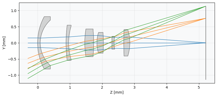
Explore the random ray distribution
First, we'll take a look at a few different pupil grids that we can trace through the system. Note that each distribution has x and y attributes, which are NumPy arrays containing the points of the distribution.
dist_rand = distribution.RandomDistribution(seed=None)
dist_rand.generate_points(num_points=100)
dist_rand.view()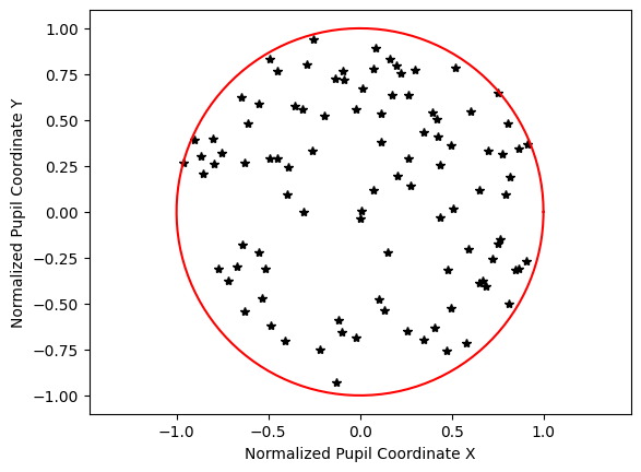
Explore the uniform ray distribution
Note that for a uniform distribution, we define the number of points along one axis.
dist_uniform = distribution.UniformDistribution()
dist_uniform.generate_points(num_points=15)
dist_uniform.view()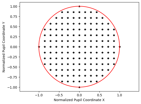
Explore the Gaussian quadrature distribution
The next distribution is the Gaussian qaudrature, which is an optimized grid for lens design based on the following paper. Essentially, this grid probes the pupil in such a way so as to accurately determine the wavefront while minimizing the number of rays traced.
G. W. Forbes, "Optical system assessment for design: numerical ray tracing in the Gaussian pupil," J. Opt. Soc. Am. A 5, 1943-1956 (1988)
dist_quad = distribution.GaussianQuadrature(is_symmetric=False)
dist_quad.generate_points(num_rings=6)
dist_quad.view()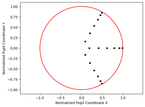
Explore the hexagonal ray distribution
The hexagonal distribution arranges rays in a symmetrical hex-grid pattern, which is well-suited for circularly symmetric systems.
dist_hex = distribution.HexagonalDistribution()
dist_hex.generate_points(num_rings=6)
dist_hex.view()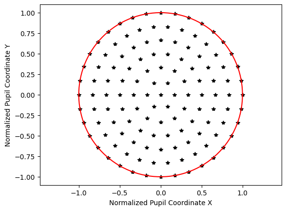
Trace on-axis rays and plot intersection positions
Now trace a random grid of rays through the reverse telephoto lens using normalized field coordinates. There are many ray properties we can extract — x, y, z intersections, L/M/N direction cosines, intensity, and optical path length. Here we plot the XY scatter of ray positions on the image plane.
rays = lens.trace(Hx=0, Hy=0, wavelength=0.55, num_rays=1024, distribution="random")

num_surfaces = lens.surface_group.num_surfaces

# take intersection points on last surface only
x_image = lens.surface_group.x[num_surfaces - 1, :]
y_image = lens.surface_group.y[num_surfaces - 1, :]

plt.scatter(x_image, y_image, s=3)
plt.axis("image")
plt.xlabel("X [mm]")
plt.ylabel("Y [mm]")
plt.title("Field Point (0, 0), $\\lambda$=0.55 µm")
plt.show()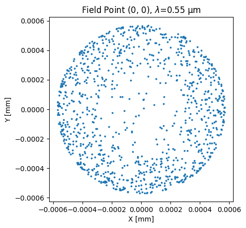
Color the scatter plot by optical path length
Retrace a hexapolar grid at 100% field and color each ray by its optical path length. This reveals the wavefront structure across the pupil.
lens.trace(Hx=0, Hy=1, wavelength=0.55, num_rays=15, distribution="hexapolar")

opd = lens.surface_group.opd[num_surfaces - 1, :]
x_image = lens.surface_group.x[num_surfaces - 1, :]
y_image = lens.surface_group.y[num_surfaces - 1, :]

plt.scatter(x_image, y_image, s=3, c=opd)
plt.xlabel("X [mm]")
plt.ylabel("Y [mm]")
plt.title("Field Point (0, 1), $\\lambda$=0.55 µm")
cbar = plt.colorbar()
cbar.ax.get_yaxis().labelpad = 25
cbar.ax.set_ylabel("Optical Path Length [mm]", rotation=270)
plt.show()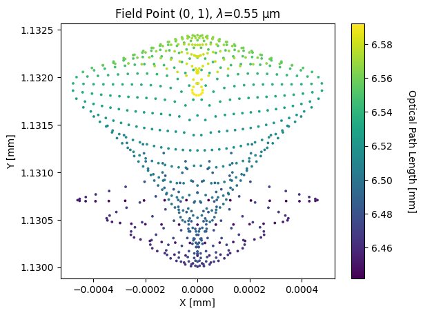
Visualize Z direction cosines at an arbitrary field point
Retrace a large uniform grid at an oblique field point and color each ray by its Z direction cosine (N). This shows how close each ray is to being parallel with the optical axis.
rays = lens.trace(
 Hx=0.825,
 Hy=0.478,
 wavelength=0.567,
 num_rays=128,
 distribution="uniform",
)

x_image = lens.surface_group.x[num_surfaces - 1, :]
y_image = lens.surface_group.y[num_surfaces - 1, :]
N = lens.surface_group.N[num_surfaces - 1, :]

plt.scatter(x_image, y_image, s=3, c=N)
plt.axis("image")
plt.xlabel("X [mm]")
plt.ylabel("Y [mm]")
plt.title("Field Point (0.825, 0.478), $\\lambda$=0.567 µm")
cbar = plt.colorbar()
cbar.ax.get_yaxis().labelpad = 25
cbar.ax.set_ylabel("Z Direction Cosine", rotation=270)
plt.xticks(rotation=45)
plt.tight_layout()
plt.show()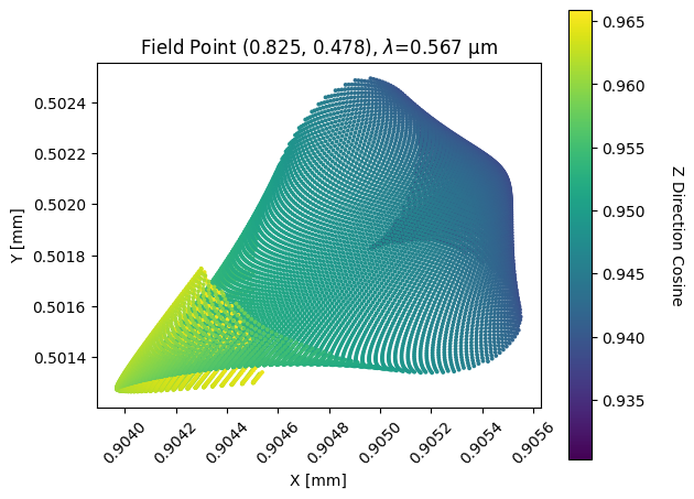
Show full code listing
import matplotlib.pyplot as plt

from optiland import distribution
from optiland.samples.objectives import ReverseTelephoto

lens = ReverseTelephoto()

lens.draw()

dist_rand = distribution.RandomDistribution(seed=None)
dist_rand.generate_points(num_points=100)
dist_rand.view()

dist_uniform = distribution.UniformDistribution()
dist_uniform.generate_points(num_points=15)
dist_uniform.view()

dist_quad = distribution.GaussianQuadrature(is_symmetric=False)
dist_quad.generate_points(num_rings=6)
dist_quad.view()

dist_hex = distribution.HexagonalDistribution()
dist_hex.generate_points(num_rings=6)
dist_hex.view()

rays = lens.trace(Hx=0, Hy=0, wavelength=0.55, num_rays=1024, distribution="random")

num_surfaces = lens.surface_group.num_surfaces

# take intersection points on last surface only
x_image = lens.surface_group.x[num_surfaces - 1, :]
y_image = lens.surface_group.y[num_surfaces - 1, :]

plt.scatter(x_image, y_image, s=3)
plt.axis("image")
plt.xlabel("X [mm]")
plt.ylabel("Y [mm]")
plt.title("Field Point (0, 0), $\\lambda$=0.55 µm")
plt.show()

lens.trace(Hx=0, Hy=1, wavelength=0.55, num_rays=15, distribution="hexapolar")

opd = lens.surface_group.opd[num_surfaces - 1, :]
x_image = lens.surface_group.x[num_surfaces - 1, :]
y_image = lens.surface_group.y[num_surfaces - 1, :]

plt.scatter(x_image, y_image, s=3, c=opd)
plt.xlabel("X [mm]")
plt.ylabel("Y [mm]")
plt.title("Field Point (0, 1), $\\lambda$=0.55 µm")
cbar = plt.colorbar()
cbar.ax.get_yaxis().labelpad = 25
cbar.ax.set_ylabel("Optical Path Length [mm]", rotation=270)
plt.show()

rays = lens.trace(
  Hx=0.825,
  Hy=0.478,
  wavelength=0.567,
  num_rays=128,
  distribution="uniform",
)

x_image = lens.surface_group.x[num_surfaces - 1, :]
y_image = lens.surface_group.y[num_surfaces - 1, :]
N = lens.surface_group.N[num_surfaces - 1, :]

plt.scatter(x_image, y_image, s=3, c=N)
plt.axis("image")
plt.xlabel("X [mm]")
plt.ylabel("Y [mm]")
plt.title("Field Point (0.825, 0.478), $\\lambda$=0.567 µm")
cbar = plt.colorbar()
cbar.ax.get_yaxis().labelpad = 25
cbar.ax.set_ylabel("Z Direction Cosine", rotation=270)
plt.xticks(rotation=45)
plt.tight_layout()
plt.show()
Conclusions
There are many other properties available, which can be seen in optiland.surfaces.SurfaceGroup.
In general, the ray information is saved in a 2D matrix with shape (num_surfaces x num_rays). All ray information is available after ray tracing, which can be configured generically. For example, various distributions can be used, but user-defined rays may also be specified. This will be discussed later.
Next tutorials
Original notebook: Tutorial_2a_Tracing_%26_Analyzing_Rays.ipynb on GitHub · ReadTheDocs