Ray Tracing

Monte Carlo Raytracing Methods

Stochastic methods for stray light and complex geometry analysis.

IntermediateRay TracingNumPy backend12 min read

Introduction

This tutorial shows one way in which Optiland can be used to run Monte Carlo simulations. Monte Carlo simulations are a computational technique used to model and analyze complex systems that involve randomness or uncertainty. They rely on repeated random sampling to estimate the behavior of a system and provide insights into the range of possible outcomes.

In a Monte Carlo simulation, a large number of random samples are generated based on the input parameters and their associated probability distributions. These samples are then used to simulate the system multiple times, allowing us to observe the distribution of outcomes and calculate various performance metrics.

Here, we will investigate how manufacturing variations of a simple singlet lens can impact performance. Note that this is a common tolerancing task.

Manufacturing variations to consider:

Lens radius of curvature
Lens index of refraction

Performance metrics to consider:

RMS spot size
RMS wavefront error

Core concepts used

np.random.normal(...)

Generates random values following a Gaussian distribution, used here to model manufacturing tolerances.

analysis.SpotDiagram(lens)

Calculates the RMS spot size for each randomized system instance.

wavefront.OPD(lens)

Retrieves the RMS wavefront error, a key metric for diffraction-limited systems.

plt.hist(...)

Visualizes the frequency of different performance outcomes across the entire population.

Step-by-step build

Import matplotlib, numpy, pandas, analysis, materials, optic, and wavefront

python

import matplotlib.pyplot as plt
import numpy as np
import pandas as pd

from optiland import analysis, materials, optic, wavefront

Sample Gaussian tolerance distributions for refractive index and radius

We choose arbitrary ranges for the lens refractive index and radius:

Refractive index: normal distribution, mean = 1.5, std=1e-3
Radius of curvature: normal distribution, mean = 100, std=0.5

In total, we will simulate 1000 systems.

python

num_systems = 1000

# set random seed for repeatability
np.random.seed(42)

refractive_index = np.random.normal(loc=1.5, scale=1e-3, size=num_systems)
radius_of_curvature = np.random.normal(loc=100, scale=0.5, size=num_systems)

Define the configurable plano-convex SingletConfigurable class

Let's define a helper class to easily generate random lenses. This is based on the simple singlet in optiland/samples/simple.py.

python

class SingletConfigurable(optic.Optic):
 """A configurable plano-convex singlet"""

 def __init__(self, radius_of_curvature, refractive_index):
     super().__init__()

     # define the material for the singlet
     ideal_material = materials.IdealMaterial(n=refractive_index, k=0)

     # add surfaces
     self.add_surface(index=0, radius=np.inf, thickness=np.inf)
     self.add_surface(
         index=1,
         thickness=5,
         radius=radius_of_curvature,
         is_stop=True,
         material=ideal_material,
     )
     self.add_surface(index=2, thickness=196.667)
     self.add_surface(index=3)

     # add aperture
     self.set_aperture(aperture_type="EPD", value=25.4)

     # add field
     self.set_field_type(field_type="angle")
     self.add_field(y=0)

     # add wavelength
     self.add_wavelength(value=0.55, is_primary=True)

Draw the first random singlet instance

Let's view the first random system.

python

lens = SingletConfigurable(radius_of_curvature[0], refractive_index[0])
lens.draw(num_rays=5)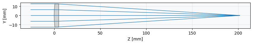

Run 1000-iteration Monte Carlo loop collecting RMS spot and wavefront error

Now we will run the Monte Carlo simulation. In each of the 1000 iterations, we generate a random system, compute the rms spot radius and rms wavefront error, and record these values for later analysis.

This code uses functionalities from the analysis and wavefront modules, which will be discussed in more detail in future tutorials.

python

rms_spot_radius = []
rms_wavefront_error = []

for k in range(num_systems):
 # generate a random singlet
 lens = SingletConfigurable(radius_of_curvature[k], refractive_index[k])

 # get value of rms spot radius at field index = 0 and wavelength index = 0
 spot = analysis.SpotDiagram(lens)
 value = spot.rms_spot_radius()[0][0]
 rms_spot_radius.append(value)

 # get rms wavefront error
 opd = wavefront.OPD(lens, field=(0, 0), wavelength=0.55)
 rms_wavefront_error.append(opd.rms())

Plot the RMS spot radius distribution

Let's plot the output distributions of our computed metrics:

python

plt.hist(rms_spot_radius, color="C0", edgecolor="k", alpha=0.8)
plt.xlabel("RMS Spot Radius (mm)")
plt.ylabel("Occurrences")
plt.show()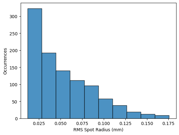

Plot the RMS wavefront error distribution

python

plt.hist(rms_wavefront_error, color="C1", edgecolor="k", alpha=0.8)
plt.xlabel("RMS Wavefront Error (waves at 0.55 µm)")
plt.ylabel("Occurrences")
plt.show()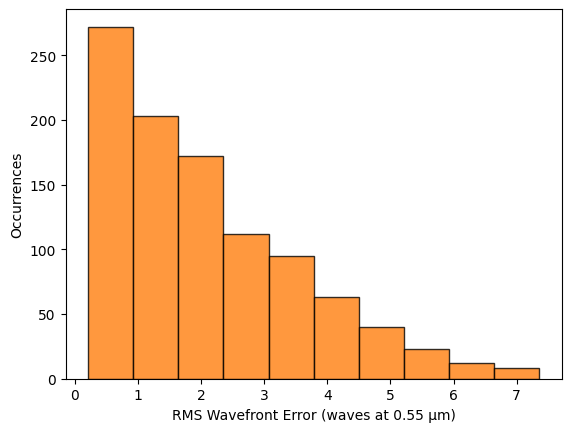

Import seaborn for correlation visualization

Let's dive deeper into the relationships by looking at the correlation matrix

python

import seaborn as sns  # pip install seaborn

Build a DataFrame from tolerance and performance results

python

df = pd.DataFrame(
 dict(
     radius_of_curvature=radius_of_curvature,
     refractive_index=refractive_index,
     rms_spot_radius=rms_spot_radius,
     rms_wavefront_error=rms_wavefront_error,
 ),
)

Compute and plot the correlation heatmap

python

# Based on: https://seaborn.pydata.org/examples/many_pairwise_correlations.html

# Compute the correlation matrix
corr = df.corr()

# Set up the matplotlib figure
f, ax = plt.subplots(figsize=(5, 3))

# Generate a custom diverging colormap
cmap = sns.diverging_palette(230, 20, as_cmap=True)

# Draw the heatmap with the mask and correct aspect ratio
sns.heatmap(corr, cmap=cmap, vmax=0.3, center=0, square=True, linewidths=0.5)

plt.show()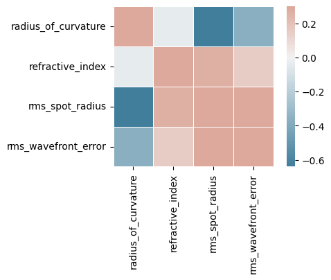

Show full code listing

python

import matplotlib.pyplot as plt
import numpy as np
import pandas as pd

from optiland import analysis, materials, optic, wavefront

num_systems = 1000

# set random seed for repeatability
np.random.seed(42)

refractive_index = np.random.normal(loc=1.5, scale=1e-3, size=num_systems)
radius_of_curvature = np.random.normal(loc=100, scale=0.5, size=num_systems)

class SingletConfigurable(optic.Optic):
  """A configurable plano-convex singlet"""

  def __init__(self, radius_of_curvature, refractive_index):
      super().__init__()

      # define the material for the singlet
      ideal_material = materials.IdealMaterial(n=refractive_index, k=0)

      # add surfaces
      self.add_surface(index=0, radius=np.inf, thickness=np.inf)
      self.add_surface(
          index=1,
          thickness=5,
          radius=radius_of_curvature,
          is_stop=True,
          material=ideal_material,
      )
      self.add_surface(index=2, thickness=196.667)
      self.add_surface(index=3)

      # add aperture
      self.set_aperture(aperture_type="EPD", value=25.4)

      # add field
      self.set_field_type(field_type="angle")
      self.add_field(y=0)

      # add wavelength
      self.add_wavelength(value=0.55, is_primary=True)

lens = SingletConfigurable(radius_of_curvature[0], refractive_index[0])
lens.draw(num_rays=5)

rms_spot_radius = []
rms_wavefront_error = []

for k in range(num_systems):
  # generate a random singlet
  lens = SingletConfigurable(radius_of_curvature[k], refractive_index[k])

  # get value of rms spot radius at field index = 0 and wavelength index = 0
  spot = analysis.SpotDiagram(lens)
  value = spot.rms_spot_radius()[0][0]
  rms_spot_radius.append(value)

  # get rms wavefront error
  opd = wavefront.OPD(lens, field=(0, 0), wavelength=0.55)
  rms_wavefront_error.append(opd.rms())

plt.hist(rms_spot_radius, color="C0", edgecolor="k", alpha=0.8)
plt.xlabel("RMS Spot Radius (mm)")
plt.ylabel("Occurrences")
plt.show()

plt.hist(rms_wavefront_error, color="C1", edgecolor="k", alpha=0.8)
plt.xlabel("RMS Wavefront Error (waves at 0.55 µm)")
plt.ylabel("Occurrences")
plt.show()

import seaborn as sns  # pip install seaborn

df = pd.DataFrame(
  dict(
      radius_of_curvature=radius_of_curvature,
      refractive_index=refractive_index,
      rms_spot_radius=rms_spot_radius,
      rms_wavefront_error=rms_wavefront_error,
  ),
)

# Based on: https://seaborn.pydata.org/examples/many_pairwise_correlations.html

# Compute the correlation matrix
corr = df.corr()

# Set up the matplotlib figure
f, ax = plt.subplots(figsize=(5, 3))

# Generate a custom diverging colormap
cmap = sns.diverging_palette(230, 20, as_cmap=True)

# Draw the heatmap with the mask and correct aspect ratio
sns.heatmap(corr, cmap=cmap, vmax=0.3, center=0, square=True, linewidths=0.5)

plt.show()

Conclusions

There are several relationships we can identify:

The RMS spot size positively correlates to the RMS wavefront error, as expected.
There is no correlation between refractive index and radius of curvature, as expected.
There is a strong negatively correlation between the RMS spot radius and the radius of curvature.

Note that these relationships are not universally true, but are based on the Monte Carlo input distributions used, the system tested, etc. With different inputs, or a different optical system, the results would undoubtedly differ.

Next tutorials

NextRaytracing AspheresModel components with non-spherical profiles for high-performance optics.RelatedTilting & De-centeringUnderstand how mechanical misalignments can also be modeled stochastically.

Original notebook: Tutorial_2c_Monte_Carlo_Raytracing.ipynb on GitHub · ReadTheDocs