Determining Lens Properties
Retrieve EFL, F/#, pupil positions, cardinal points, and paraxial ray data from an optical system.
Introduction
This tutorial shows how to inspect the main first-order properties of a lens in Optiland using the built-in Cooke Triplet sample. You will retrieve focal quantities, principal and nodal plane locations, pupil diameters and positions, the optical invariant, and the paraxial marginal and chief rays.
By the end, you will know where to look in the lens.paraxial interface when you need quick optical diagnostics without moving to full ray analysis.
Core concepts used
Step-by-step walkthrough
Load and preview the Cooke Triplet
Import the built-in Cooke Triplet sample, instantiate it, and draw the layout to establish a geometric picture of the lens before reading its first-order properties.
from optiland.samples.objectives import CookeTriplet

lens = CookeTriplet()
lens.draw()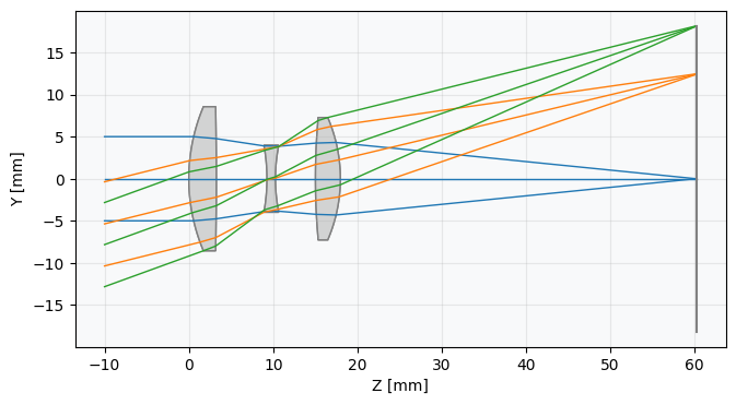
Read focal, principal, and nodal data
Query the most common cardinal-point quantities, including front and back focal lengths, focal points, principal planes, and nodal planes.
print(f"Front focal length: {lens.paraxial.f1():.1f} mm")
print(f"Focal length: {lens.paraxial.f2():.1f} mm")
print(f"Front focal point: {lens.paraxial.F1():.1f} mm")
print(f"Back focal point: {lens.paraxial.F2():.1f} mm")
print(f"Front principal plane: {lens.paraxial.P1():.1f} mm")
print(f"Back principal plane: {lens.paraxial.P2():.1f} mm")
print(f"Front nodal plane: {lens.paraxial.N1():.1f} mm")
print(f"Back nodal plane: {lens.paraxial.N2():.1f} mm")Measure entrance and exit pupil diameters
For object-space quantities, Optiland measures positions relative to the first lens surface. Image-space quantities are measured relative to the image surface.
print(f"Entrance pupil diameter: {lens.paraxial.EPD():.1f} mm")
print(f"Exit pupil diameter: {lens.paraxial.XPD():.1f} mm")Measure entrance and exit pupil locations
After checking pupil sizes, retrieve the longitudinal locations of the entrance and exit pupils.
print(f"Entrance pupil position: {lens.paraxial.EPL():.1f} mm")
print(f"Exit pupil position: {lens.paraxial.XPL():.1f} mm")Compute F-number, magnification, and invariant
Magnification is usually most meaningful for finite-conjugate systems, but it is included here as a simple illustration alongside the image-space F-number and optical invariant.
print(f"Image-space F-Number: {lens.paraxial.FNO():.1f}")
print(f"Magnification: {lens.paraxial.magnification():.1f}")
print(f"Invariant: {lens.paraxial.invariant():.3f}")Inspect the marginal ray across the system
Print the paraxial marginal ray height and slope at each surface to see how the edge-of-aperture ray evolves through the lens.
print("Marginal Ray: ")

ya, ua = lens.paraxial.marginal_ray()
for k in range(len(ya)):
print(f"\tSurface {k}: y = {ya[k, 0]:.3f}, u = {ua[k, 0]:.3f}")Inspect the chief ray across the system
Finally, print the paraxial chief ray height and slope at each surface to understand how the field ray propagates through the system.
print("Chief Ray: ")

yb, ub = lens.paraxial.chief_ray()
for k in range(len(yb)):
    print(f"\tSurface {k}: y = {yb[k, 0]:.3f}, u = {ub[k, 0]:.3f}")
Show full code listing
from optiland.samples.objectives import CookeTriplet

lens = CookeTriplet()

lens.draw()

print(f"Front focal length: {lens.paraxial.f1():.1f} mm")
print(f"Focal length: {lens.paraxial.f2():.1f} mm")
print(f"Front focal point: {lens.paraxial.F1():.1f} mm")
print(f"Back focal point: {lens.paraxial.F2():.1f} mm")
print(f"Front principal plane: {lens.paraxial.P1():.1f} mm")
print(f"Back principal plane: {lens.paraxial.P2():.1f} mm")
print(f"Front nodal plane: {lens.paraxial.N1():.1f} mm")
print(f"Back nodal plane: {lens.paraxial.N2():.1f} mm")

print(f"Entrance pupil diameter: {lens.paraxial.EPD():.1f} mm")
print(f"Exit pupil diameter: {lens.paraxial.XPD():.1f} mm")

print(f"Entrance pupil position: {lens.paraxial.EPL():.1f} mm")
print(f"Exit pupil position: {lens.paraxial.XPL():.1f} mm")

print(f"Image-space F-Number: {lens.paraxial.FNO():.1f}")
print(f"Magnification: {lens.paraxial.magnification():.1f}")
print(f"Invariant: {lens.paraxial.invariant():.3f}")

print("Marginal Ray: ")

ya, ua = lens.paraxial.marginal_ray()
for k in range(len(ya)):
    print(f"\tSurface {k}: y = {ya[k, 0]:.3f}, u = {ua[k, 0]:.3f}")

print("Chief Ray: ")

yb, ub = lens.paraxial.chief_ray()
for k in range(len(yb)):
    print(f"\tSurface {k}: y = {yb[k, 0]:.3f}, u = {ub[k, 0]:.3f}")
Conclusions
The paraxial interface gives a compact first-order summary of an optical system: focal properties, pupil data, cardinal planes, and paraxial ray behavior. This makes it a useful entry point when you want to inspect a design quickly before moving to full tracing, aberration analysis, or optimization.
Next tutorials
Original notebook: Tutorial_1b_Lens_Properties.ipynb on GitHub · ReadTheDocs