Optimization

Simple Optimization

Automatically refine lens parameters to minimize aberrations.

IntermediateOptimizationNumPy backend12 min read

Introduction

This tutorial shows how to optimize optical systems in Optiland. In this example, we will optimize a singlet.

Core concepts used

optimization.OptimizationProblem()

The container for your design task. it holds all the "knobs" (variables) and "goals" (operands).

problem.add_variable(...)

Defines which lens parameters the computer is allowed to change (e.g., radius, thickness, material).

problem.add_operand(...)

Sets a target for the optimizer. Examples include f2 (focal length) or OPD_difference (wavefront quality).

optimization.OptimizerGeneric(problem)

A standard numerical solver using local search algorithms to minimize the merit function value.

Step-by-step build

Import libraries

python

import numpy as np

from optiland import analysis, optic, optimization, wavefront

Build the initial singlet and inspect layout

We first define a simple singlet. We will make it double convex and will define a few fields and wavelengths.

python

lens = optic.Optic()

# add surfaces
lens.add_surface(index=0, thickness=np.inf)
lens.add_surface(index=1, thickness=5, radius=100, is_stop=True, material="N-SF11")
lens.add_surface(index=2, thickness=59, radius=-1000)
lens.add_surface(index=3)

# add aperture
lens.set_aperture(aperture_type="EPD", value=25)

# add field
lens.set_field_type(field_type="angle")
lens.add_field(y=0.0)
lens.add_field(y=0.7)
lens.add_field(y=1.0)

# add wavelength
lens.add_wavelength(value=0.4861)
lens.add_wavelength(value=0.5876, is_primary=True)
lens.add_wavelength(value=0.6563)

lens.update_paraxial()

python

le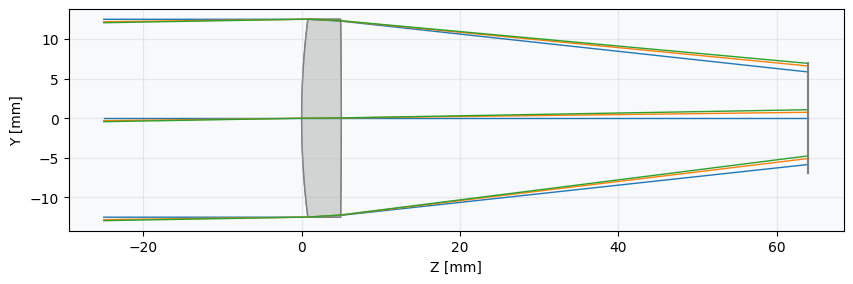ns.draw()

Define the optimisation problem

Now, we need to define the optimization problem, which contains all information about the variables and operands.

In particular, we will optimize for minimal optical path difference for each field. We will also add an operand to specify the focal length at 100 mm. As for variables, we will let the lens radii vary and the distance from the lens to the image plane. Once defined, we can view all information related to the optimization problem using the 'info' method.

There are many operand types available, which can be seen in optiland.operand. Variable options can be seen in optiland.variable,

python

problem = optimization.OptimizationProblem()

for wave in lens.wavelengths.get_wavelengths():
 for Hx, Hy in lens.fields.get_field_coords():
     input_data = {
         "optic": lens,
         "Hx": Hx,
         "Hy": Hy,
         "num_rays": 3,
         "wavelength": wave,
         "distribution": "gaussian_quad",
     }
     problem.add_operand(
         operand_type="OPD_difference",
         target=0,
         weight=1,
         input_data=input_data,
     )

problem.add_operand(
 operand_type="f2",
 target=100,
 weight=10,
 input_data={"optic": lens},
)

problem.add_variable(lens, "thickness", surface_number=2, min_val=0, max_val=1000)
problem.add_variable(lens, "radius", surface_number=1, min_val=-1000, max_val=1000)
problem.add_variable(lens, "radius", surface_number=2, min_val=-1000, max_val=1000)

problem.info()

Create the optimizer

We now need to define an optimizer, which will take the optimization problem as an input. We choose the standard "generic" optimizer, but there are many other options, including a least squares optimizer.

Note that the generic optimizer simply utilizes scipy.optimize.minimize.

python

optimizer = optimization.OptimizerGeneric(problem)

# We can also use a least squares optimizer as follows:
# optimizer = optimization.LeastSquares(problem)

Run the optimiser and review results

We can now simply call the optimizer.

python

res = optimizer.optimize()

If we now view the optimization problem info, we can see that we've significantly improved the system (>99.9%)

python

problem.info()

Inspect the optimised lens layout

And when we view the lens, we see that it properly focuses the light on our image plane.

python

lens.draw()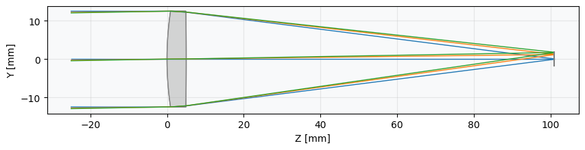

Analyse ray aberrations

Let's look at a few other common analyes:

python

fan = analysis.RayFan(lens)
fan.view()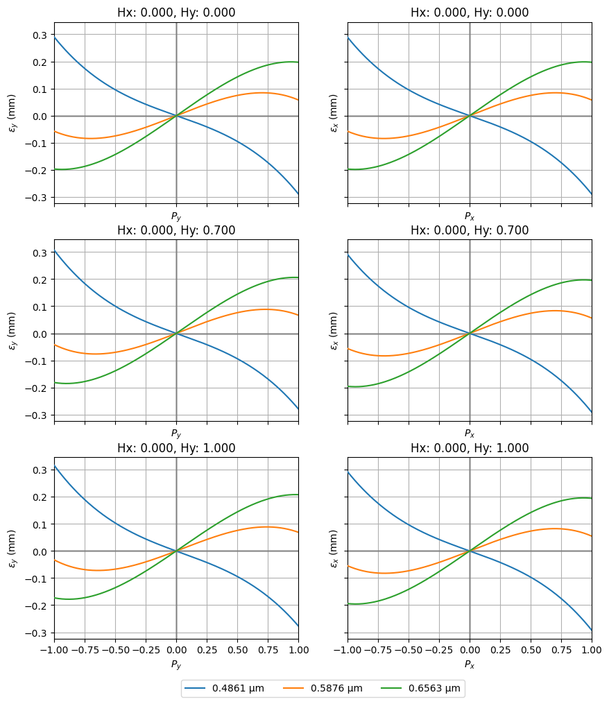

python

spot = analysis.SpotDiagram(lens)
spot.view()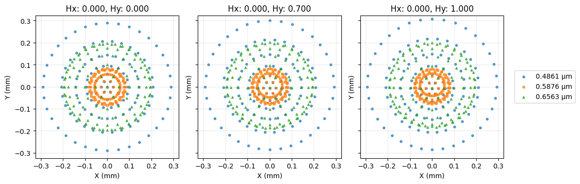

Visualise the wavefront OPD

python

opd = wavefront.OPD(lens, field=(0, 1), wavelength=0.55)
opd.view(projection="2d", num_points=512)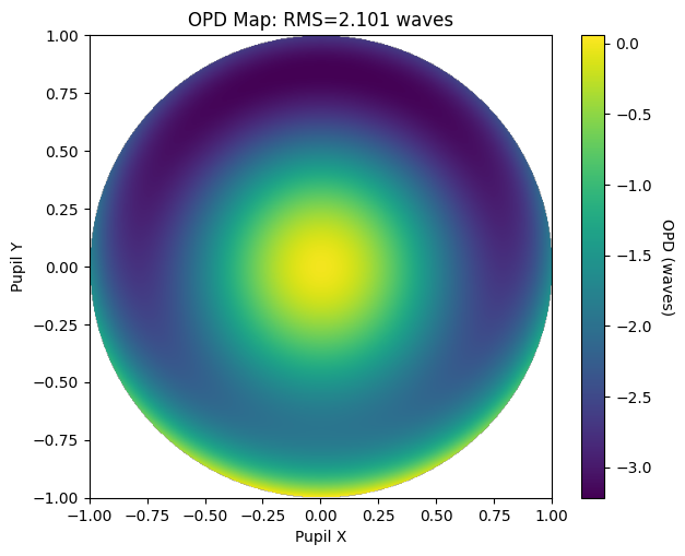

Show full code listing

python

import numpy as np

from optiland import analysis, optic, optimization, wavefront

lens = optic.Optic()

# add surfaces
lens.add_surface(index=0, thickness=np.inf)
lens.add_surface(index=1, thickness=5, radius=100, is_stop=True, material="N-SF11")
lens.add_surface(index=2, thickness=59, radius=-1000)
lens.add_surface(index=3)

# add aperture
lens.set_aperture(aperture_type="EPD", value=25)

# add field
lens.set_field_type(field_type="angle")
lens.add_field(y=0.0)
lens.add_field(y=0.7)
lens.add_field(y=1.0)

# add wavelength
lens.add_wavelength(value=0.4861)
lens.add_wavelength(value=0.5876, is_primary=True)
lens.add_wavelength(value=0.6563)

lens.update_paraxial()

lens.draw()

problem = optimization.OptimizationProblem()

for wave in lens.wavelengths.get_wavelengths():
  for Hx, Hy in lens.fields.get_field_coords():
      input_data = {
          "optic": lens,
          "Hx": Hx,
          "Hy": Hy,
          "num_rays": 3,
          "wavelength": wave,
          "distribution": "gaussian_quad",
      }
      problem.add_operand(
          operand_type="OPD_difference",
          target=0,
          weight=1,
          input_data=input_data,
      )

problem.add_operand(
  operand_type="f2",
  target=100,
  weight=10,
  input_data={"optic": lens},
)

problem.add_variable(lens, "thickness", surface_number=2, min_val=0, max_val=1000)
problem.add_variable(lens, "radius", surface_number=1, min_val=-1000, max_val=1000)
problem.add_variable(lens, "radius", surface_number=2, min_val=-1000, max_val=1000)

problem.info()

optimizer = optimization.OptimizerGeneric(problem)

# We can also use a least squares optimizer as follows:
# optimizer = optimization.LeastSquares(problem)

res = optimizer.optimize()

problem.info()

lens.draw()

fan = analysis.RayFan(lens)
fan.view()

spot = analysis.SpotDiagram(lens)
spot.view()

opd = wavefront.OPD(lens, field=(0, 1), wavelength=0.55)
opd.view(projection="2d", num_points=512)

Conclusions

Defined a least-squares optimization problem by specifying operands for effective focal length, Seidel aberrations (S1–S4), and RMS spot size, then adding surface radii as free variables.
Used OptimizerGeneric with the least_squares method to drive the singlet toward a diffraction-limited design in a single call.
Inspected convergence with problem.info() and confirmed the optimized prescription numerically.
Verified the improved performance visually using RayFan, SpotDiagram, and a 2D OPD map, observing the reduction in aberration residuals compared to the starting design.

Next tutorials

NextAdvanced OptimizationUse global search and multi-configuration solvers for complex designs.RelatedZernike DecompositionUnderstand the aberrations that the optimizer is trying to eliminate.

Original notebook: Tutorial_5a_Simple_Optimization.ipynb on GitHub · ReadTheDocs