Tolerancing, Sensitivity Analyses
Analyze how small manufacturing errors impact the performance of your design.
Introduction
In this tutorial, we will explore the process of tolerancing an optical system in Optiland via sensitivity analysis. Tolerancing is a crucial aspect of optical design, ensuring that the system performs adequately despite manufacturing imperfections. Sensitivity analysis helps in understanding how variations in design parameters affect the overall performance of the optical system.
Tolerancing in Optiland requires 4 key components:
- Optic - the optical system to be analyzed.
- Operands - the metrics which are assessed e.g., wavefront error.
- Perturbations - the variations applied to the optic or a surface of an optic e.g., surface tilt.
- Compensators - a parameter of the optical system that can be adjusted to counteract the effects of a perturbation.
In this example, we will apply various perturbations to our optic, one at a time, while monitoring various metrics, or operands. We will perform a sensitivity analysis, which will show the variation in each metric (operand) as a function of each perturbation. In this case, all perturbations are applied independently.
Core concepts used
Step-by-step build
Import Tolerancing Classes
from optiland.samples.objectives import CookeTriplet
from optiland.tolerancing import RangeSampler, SensitivityAnalysis, TolerancingInitialize the Cooke Triplet Optic
- Defining the tolerancing object:
The core of tolerancing in Optiland is the Tolerancing class. This class contains all operands, perturbations and compensators that are used during a tolerancing exercise. We start by defining a Cooke triplet and passing it to our Tolerancing class.
optic = CookeTriplet()Create the Tolerancing Object
tolerancing = Tolerancing(optic)Add Radius of Curvature Perturbation
- Adding perturbations
Each tolerancing object contains perturbations, or variations that are applied to the optic during a tolerancing analysis. Each perturbation requires a value that should be applied to the perturbation. For example, we may wish to tilt the first surface by 0.01 radians. The values of a given perturbation are specified via "samplers", which provide the perturbation value in each iteration. We define a "RangeSampler", in which perturbation values are defined in a linear range from a "start" value to a "end" value over a given number of "steps".
For the first perturbation, we wish to specify the following properties:
- Variation in radius of curvature of first surface of lens
- Variation occurs from 15 mm to 30 mm over 128 steps
This is defined and added to our tolerancing instance as follows:
sampler = RangeSampler(start=15, end=30, steps=128)
tolerancing.add_perturbation("radius", sampler, surface_number=1)Add Surface X-Tilt Perturbation
For the next perturbation, we will apply a variation of x-tilt to the first surface:
sampler = RangeSampler(start=-0.05, end=0.05, steps=128)  # radians
tolerancing.add_perturbation("tilt", sampler, surface_number=1, axis="x")Add Surface Thickness Perturbation
For the last perturbation, we will vary the thickness of our first lens (at surface 1):
sampler = RangeSampler(start=2, end=5, steps=128)
tolerancing.add_perturbation("thickness", sampler, surface_number=1)Add Focal Length, Spot Size, and OPD Operands
- Adding operands
When we apply perturbations, we want to monitor various performance metrics. Here, we will monitor:
- focal length
- RMS spot size
- mean OPD difference
The syntax used here follows that used in the optimization module when variables are defined. In general, we pass the following arguments to the "add_operand" method to create a new operand:
- operand type - see optiland.optimization.operand for complete list of options.
- input_data - a dictionary containing the optic instance at a minimum, and generally other parameters related to the operand, such as wavelength.
- target (optional) - if an operand has a target, we may specify it here. This is only used when we apply compensation, or optimize the system to counteract perturbations.
- weight (optional) - if an operand is more important than others, it may be given a larger weight during compensation.
We define the 3 operands as follows:
input_data = {"optic": optic}
tolerancing.add_operand("f2", input_data)

input_data = {
 "optic": optic,
 "surface_number": -1,
 "Hx": 0,
 "Hy": 0.0,
 "wavelength": 0.55,
 "num_rays": 5,
}  # surface_number=-1 means the last surface
tolerancing.add_operand("rms_spot_size", input_data, target=0)

input_data = {"optic": optic, "Hx": 0, "Hy": 1, "wavelength": 0.55, "num_rays": 5}
tolerancing.add_operand("OPD_difference", input_data)Create the SensitivityAnalysis Object
- Run sensitivity analysis
The next step is to pass our tolerancing variable to a "SensitivityAnalysis" instance. This class performs all sensitivity operations, saves the results, and provides an interface to view the results.
sensitivity_analysis = SensitivityAnalysis(tolerancing)Run the Sensitivity Analysis
And we can now run the analysis. The duration of the analysis will depend on the number of operands, perturbations and their ranges, as well as whether compensators are applied. On the author's machine, this analysis takes a couple seconds (for ≈400 evaluations in total).
sensitivity_analysis.run()Visualize Perturbation vs. Operand Plots
- View and analyze results
We can call the "view" method of SensitivityAnalysis to show effect of the perturbations on the operands:
sensitivity_analysis.view()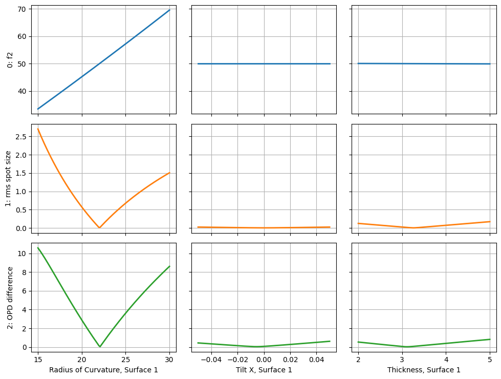
Retrieve Results as a DataFrame
As we defined 3 operands and 3 perturbations, we see a collection of 9 (3x3) plots. The rows represent the operands and the columns represent the perturbations. A few relationships we can observe:
- the strongest effect by far is perturbation of the radius of curvature
- the RMS spot size and OPD difference are a minimum at the nominal radius of curvature value (≈22mm)
- tilting or changing the thickness of surface 1 has little impact on the focal length
- tilt has a small impact on the OPD difference, with a minimum near 0 radians
Lastly, if we wish to further analyze the results, we can retrieve all results via the "get_results" method, which returns a pandas DataFrame.
df = sensitivity_analysis.get_results()Inspect the First Rows
df.head()Summarize Descriptive Statistics
df.describe()Export Results to CSV
We may also save the results to a csv file:
df.to_csv("sensitivity_analysis.csv")Show full code listing
from optiland.samples.objectives import CookeTriplet
from optiland.tolerancing import RangeSampler, SensitivityAnalysis, Tolerancing

optic = CookeTriplet()

tolerancing = Tolerancing(optic)

sampler = RangeSampler(start=15, end=30, steps=128)
tolerancing.add_perturbation("radius", sampler, surface_number=1)

sampler = RangeSampler(start=-0.05, end=0.05, steps=128)  # radians
tolerancing.add_perturbation("tilt", sampler, surface_number=1, axis="x")

sampler = RangeSampler(start=2, end=5, steps=128)
tolerancing.add_perturbation("thickness", sampler, surface_number=1)

input_data = {"optic": optic}
tolerancing.add_operand("f2", input_data)

input_data = {
  "optic": optic,
  "surface_number": -1,
  "Hx": 0,
  "Hy": 0.0,
  "wavelength": 0.55,
  "num_rays": 5,
}  # surface_number=-1 means the last surface
tolerancing.add_operand("rms_spot_size", input_data, target=0)

input_data = {"optic": optic, "Hx": 0, "Hy": 1, "wavelength": 0.55, "num_rays": 5}
tolerancing.add_operand("OPD_difference", input_data)

sensitivity_analysis = SensitivityAnalysis(tolerancing)

sensitivity_analysis.run()

sensitivity_analysis.view()

df = sensitivity_analysis.get_results()

df.head()

df.describe()

df.to_csv("sensitivity_analysis.csv")
Conclusions
Conclusions
-
This tutorial demonstrated the basics of tolerancing in Optiland.
-
Tolerancers in Optiland require:
- an optic
- operand(s)
- perturbation(s)
- (optional) compensator(s)
-
A sensitivity analysis can be performed by first defining a tolerancing object, then passing it to SensitivityAnalysis and calling the "run" method.
-
The results of a sensitivity analysis can be retrieved as a pandas DataFrame and saved for further analysis.
Next tutorials
Original notebook: Tutorial_8a_Tolerancing_Sensitivity_Analysis.ipynb on GitHub · ReadTheDocs