Tolerancing, Monte Carlo
Simulate thousands of random builds to predict manufacturing yield.
Introduction
In this tutorial, we will continue to explore the tolerancing capabilities of Optiland and will introduce Monte Carlo analysis. Monte Carlo analysis involves simulating a large number of random variations of an optical system, which helps to understand the statistical distribution of potential performance outcomes for a system. It is particularly valuable for understanding the impact of manufacturing defects and environmental conditions.
The Monte Carlo analysis in Optiland is fundamentally similar to the sensitivity analysis, which was introduced in tutorial 8a. We require the following components to perform a Monte Carlo analysis:
- Optic - the optical system to be analyzed.
- Operands - the metrics which are assessed e.g., wavefront error.
- Perturbations - the variations applied to the optic or a surface of an optic e.g., surface tilt.
- Compensators - a parameter of the optical system that can be adjusted to counteract the effects of a perturbation.
In this example, we will perform a Monte Carlo analysis on a Cooke triplet to understand how common variations, such as surface decenter and tilt, can impact the optical performance.
Core concepts used
scale is the manufacturing standard deviation.Step-by-step build
Import Monte Carlo Classes
from optiland.samples.objectives import CookeTriplet
from optiland.tolerancing.core import Tolerancing
from optiland.tolerancing.monte_carlo import MonteCarlo
from optiland.tolerancing.perturbation import DistributionSamplerInitialize the Cooke Triplet Optic
- Defining the tolerancing object
The first step is to define our optic and pass it to a Tolerancing object.
optic = CookeTriplet()Create the Tolerancing Object
tolerancing = Tolerancing(optic)Add Random Tilt and Decenter Perturbations
The Monte Carlo anlaysis requires that we apply random perturbations to optical properties of our system. We will apply both random tilt and random decenter to every surface of the triplet, so 6 surfaces in total. We will apply perturbations to every surface and in both the x and y axes.
Properties for tilt perturbation:
- Normal distribution, mean = 0, standard deviation = 0.01 radians
Properties for decenter perturbation:
-
Normal distribution, mean = 0, standard deviation = 0.1 mm
python# loop through all surfaces and add perturbations for k in range(1, 7): # X-tilt sampler = DistributionSampler("normal", loc=0, scale=0.01) tolerancing.add_perturbation("tilt", sampler, surface_number=k, axis="x") # Y-tilt sampler = DistributionSampler("normal", loc=0, scale=0.01) tolerancing.add_perturbation("tilt", sampler, surface_number=k, axis="y") # X-decenter sampler = DistributionSampler("normal", loc=0, scale=0.1) tolerancing.add_perturbation("decenter", sampler, surface_number=k, axis="x") # Y-decenter sampler = DistributionSampler("normal", loc=0, scale=0.1) tolerancing.add_perturbation("decenter", sampler, surface_number=k, axis="y")
Add Spot Size, OPD, and Y-Intercept Operands
- Adding operands
We wish to monitor the impact of perturbations on our triplet. We choose to monitor the following metrics:
- RMS spot size for (Hx, Hy) = (0, 1) field
- mean OPD difference for (Hx, Hy) = (0, 1) field
- real y-intercept on image plane for (Hx, Hy) = (0, 1) field
The syntax used here follows that used in the optimization module when variables are defined. In general, we pass the following arguments to the "add_operand" method to create a new operand:
- operand type - see optiland.optimization.operand for complete list of options.
- input_data - a dictionary containing the optic instance at a minimum, and generally other parameters related to the operand, such as wavelength.
- target (optional) - if an operand has a target, we may specify it here. This is only used when we apply compensation, or optimize the system to counteract perturbations.
- weight (optional) - if an operand is more important than others, it may be given a larger weight during compensation.
We define the 3 operands as follows:
input_data = {
"optic": optic,
"surface_number": -1,
"Hx": 0,
"Hy": 1,
"wavelength": 0.55,
"num_rays": 5,
}
tolerancing.add_operand("rms_spot_size", input_data, target=0)
input_data = {"optic": optic, "Hx": 0, "Hy": 1, "wavelength": 0.55, "num_rays": 5}
tolerancing.add_operand("OPD_difference", input_data)
input_data = {
"optic": optic,
"surface_number": -1,
"Hx": 0,
"Hy": 1,
"Px": 0,
"Py": 0,
"wavelength": 0.55,
}
tolerancing.add_operand("real_y_intercept", input_data)Create the MonteCarlo Object
- Run Monte Carlo analysis
We are now ready to run our Monte Carlo analysis. We first define our Monte Carlo analysis:
monte_carlo = MonteCarlo(tolerancing)Run 1,000 Monte Carlo Iterations
We can then run our Monte Carlo analysis. We choose to run 1000 iterations.
monte_carlo.run(num_iterations=1000)Plot Operand Histograms
- View and analyze results
There are several ways to view the output data of a Monte Carlo analysis:
-
Plot the distributions of the performance metrics
-
Plot the cumulative distribution function (CDF) of the metrics
-
Plot a heatmap showing the correlations between the perturbations and the metrics
pythonmonte_carlo.view_histogram(kde=False)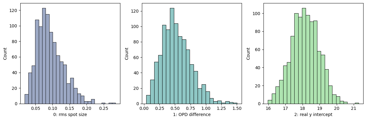
Plot Cumulative Distribution Functions
monte_carlo.view_cdf()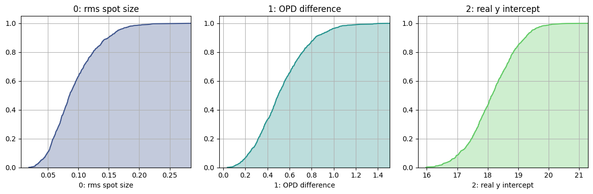
Plot Perturbation Correlation Heatmap
monte_carlo.view_heatmap(vmin=-0.2, vmax=0.2, figsize=(10, 10))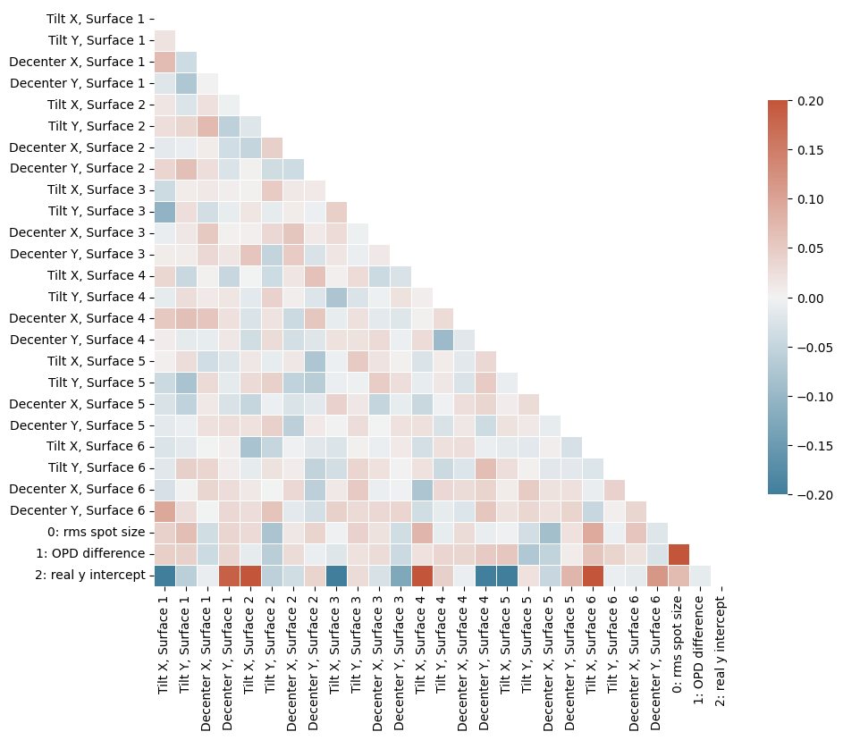
Retrieve Results as a DataFrame
The heatmap gives an indication of the correlation between the metrics and the various pertrurbations applied. The strongest correlations exist between the real y-intercept and several of the surface tilts and decenters.
As with the sensitivity analysis, we can also retrieve the Monte Carlo results for further analysis:
df = monte_carlo.get_results()Inspect the First Rows
df.head()Show full code listing
from optiland.samples.objectives import CookeTriplet
from optiland.tolerancing.core import Tolerancing
from optiland.tolerancing.monte_carlo import MonteCarlo
from optiland.tolerancing.perturbation import DistributionSampler
optic = CookeTriplet()
tolerancing = Tolerancing(optic)
# loop through all surfaces and add perturbations
 for k in range(1, 7):
     # X-tilt
     sampler = DistributionSampler("normal", loc=0, scale=0.01)
     tolerancing.add_perturbation("tilt", sampler, surface_number=k, axis="x")

     # Y-tilt
     sampler = DistributionSampler("normal", loc=0, scale=0.01)
     tolerancing.add_perturbation("tilt", sampler, surface_number=k, axis="y")

     # X-decenter
     sampler = DistributionSampler("normal", loc=0, scale=0.1)
     tolerancing.add_perturbation("decenter", sampler, surface_number=k, axis="x")

     # Y-decenter
     sampler = DistributionSampler("normal", loc=0, scale=0.1)
     tolerancing.add_perturbation("decenter", sampler, surface_number=k, axis="y")
input_data = {
 "optic": optic,
 "surface_number": -1,
 "Hx": 0,
 "Hy": 1,
 "wavelength": 0.55,
 "num_rays": 5,
}
tolerancing.add_operand("rms_spot_size", input_data, target=0)

input_data = {"optic": optic, "Hx": 0, "Hy": 1, "wavelength": 0.55, "num_rays": 5}
tolerancing.add_operand("OPD_difference", input_data)

input_data = {
 "optic": optic,
 "surface_number": -1,
 "Hx": 0,
 "Hy": 1,
 "Px": 0,
 "Py": 0,
 "wavelength": 0.55,
}
tolerancing.add_operand("real_y_intercept", input_data)
monte_carlo = MonteCarlo(tolerancing)
monte_carlo.run(num_iterations=1000)
monte_carlo.view_histogram(kde=False)
monte_carlo.view_cdf()
monte_carlo.view_heatmap(vmin=-0.2, vmax=0.2, figsize=(10, 10))
df = monte_carlo.get_results()
df.head()Conclusions
Conclusions
- This tutorial demonstrated Monte Carlo analyses in Optiland.
- Monte Carlo analysis is a statistical technique to explore possible system performance variations due to manufacturing tolerances or environmental conditions.
- Several plotting functions are available via the Monte Carlo analysis object, including plotting of distributions, CDFs, and heatmaps.
Next tutorials
Original notebook: Tutorial_8b_Monte_Carlo_Analysis.ipynb on GitHub · ReadTheDocs