Thin Film Tolerance Analysis
Perform sensitivity analysis and Monte Carlo simulations to evaluate the manufacturability of thin film designs.
Introduction
This tutorial demonstrates sensitivity analysis and Monte Carlo simulation for thin film stacks, applied to a realistic 7-layer broadband AR coating on N-BK7 glass (designed via needle synthesis in Tutorial 6h).
Manufacturing variations in layer thickness shift spectral performance. We answer:
- Which layers are most critical? (sensitivity analysis)
- What is the expected yield under realistic tolerances? (Monte Carlo)
- What does the worst-case reflectance spectrum look like? (spectral tolerance band)
Core concepts used
Step-by-step build
Import libraries and tolerancing tools
import numpy as np
import matplotlib.pyplot as plt
from optiland.materials import Material, IdealMaterial
from optiland.thin_film import ThinFilmStack
from optiland.thin_film.optimization.operand.thin_film import ThinFilmOperand
from optiland.thin_film.tolerancing import (
 ThinFilmTolerancing,
 ThinFilmSensitivityAnalysis,
 ThinFilmMonteCarlo,
)
from optiland.tolerancing.perturbation import RangeSampler, DistributionSampler1. Nominal design 7-layer broadband AR on N-BK7
This is the optimized design from Tutorial 6h (needle synthesis). It uses alternating MgF2/Al2O3 layers to achieve R < 1% across 420–680 nm.
air = IdealMaterial(n=1.0)
nbk7 = Material("N-BK7")
mgf2 = Material("MgF2", reference="Dodge-o")
al2o3 = Material("Al2O3", reference="Malitson")

# 7-layer design from needle synthesis (Tutorial 6h)
stack = ThinFilmStack(incident_material=air, substrate_material=nbk7)
stack.add_layer_nm(mgf2, 94.6, name="MgF2")
stack.add_layer_nm(al2o3, 319.7, name="Al2O3")
stack.add_layer_nm(mgf2, 17.7, name="MgF2")
stack.add_layer_nm(al2o3, 196.1, name="Al2O3")
stack.add_layer_nm(mgf2, 26.3, name="MgF2")
stack.add_layer_nm(al2o3, 170.9, name="Al2O3")
stack.add_layer_nm(mgf2, 190.4, name="MgF2")
print(stack)Plot the nominal reflectance spectrum
wl_plot = np.linspace(400, 720, 300)
R_nominal = np.array([ThinFilmOperand.reflectance(stack, wl) for wl in wl_plot])

fig, ax = plt.subplots(figsize=(9, 5))
ax.plot(wl_plot, R_nominal * 100, "-", color="steelblue", linewidth=2, label="Nominal")
ax.axhline(1.0, color="red", linestyle="--",
        linewidth=1, alpha=0.7, label="Spec: R < 1%")
ax.axvspan(420, 680, alpha=0.06, color="blue", label="Target band")
ax.set_xlabel("Wavelength (nm)")
ax.set_ylabel("Reflectance (%)")
ax.set_title("Nominal Design — 7-Layer Broadband AR on N-BK7")
ax.set_ylim(0, 4)
ax.legend()
ax.grid(True, alpha=0.3)
fig.tight_layout();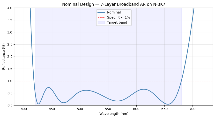
2. Sensitivity Analysis
We perturb each layer thickness individually by ±3% (typical for ion-beam sputtering) and observe how reflectance at blue (450 nm), green (550 nm), and red (650 nm) responds. This reveals which of the 7 layers are most critical to control.
tol = ThinFilmTolerancing(stack)

# Operands: reflectance at three key wavelengths
tol.add_operand("R", 450.0)
tol.add_operand("R", 550.0)
tol.add_operand("R", 650.0)

# ±3% thickness perturbation on each of the 7 layers
for i in range(7):
 tol.add_perturbation(i, "thickness", RangeSampler(-0.03, 0.03, 13))

sa = ThinFilmSensitivityAnalysis(tol)
sa.run()

fig, axes = sa.view()
fig.suptitle("Sensitivity: R vs. Layer Thickness Perturbation (±3%)", y=1.02)
fig.tight_layout();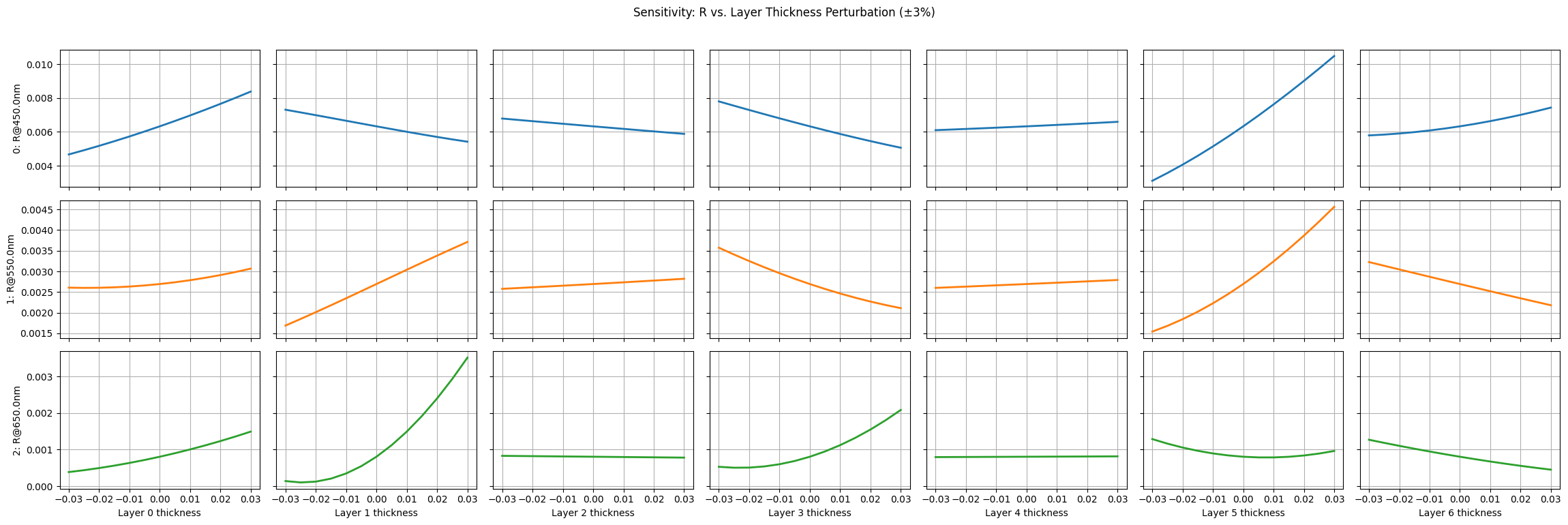
Quantify sensitivity ranges per layer
# Identify which layers have the steepest sensitivity slopes
df_sa = sa.get_results()
operand_cols = [
 c for c in df_sa.columns
 if c.startswith("0:") or c.startswith("1:") or c.startswith("2:")
]

print("Sensitivity range (max - min reflectance) per layer:")
for ptype in df_sa["perturbation_type"].unique():
 mask = df_sa["perturbation_type"] == ptype
 ranges = df_sa.loc[mask, operand_cols].max() - df_sa.loc[mask, operand_cols].min()
 worst = ranges.max()
print(f" {ptype}: max ΔR = {worst*100:.3f}%")3. Monte Carlo Analysis
We apply normally-distributed thickness errors (2% std, relative) to all 7 layers simultaneously over 500 trials. This models realistic sputtering variability.
tol_mc = ThinFilmTolerancing(stack)

# Operands: reflectance at 5 wavelengths across the band
for wl in [430.0, 480.0, 550.0, 620.0, 670.0]:
 tol_mc.add_operand("R", wl)

# 2% std thickness perturbation on all 7 layers
for i in range(7):
 tol_mc.add_perturbation(
     i, "thickness",
     DistributionSampler("normal", seed=100 + i, loc=0.0, scale=0.02),
 )

mc = ThinFilmMonteCarlo(tol_mc)
mc.run(num_iterations=500)
print(f"Monte Carlo complete: {len(mc.get_results())} trials")Plot reflectance distributions and yield CDF
fig, axes = mc.view_histogram(kde=True)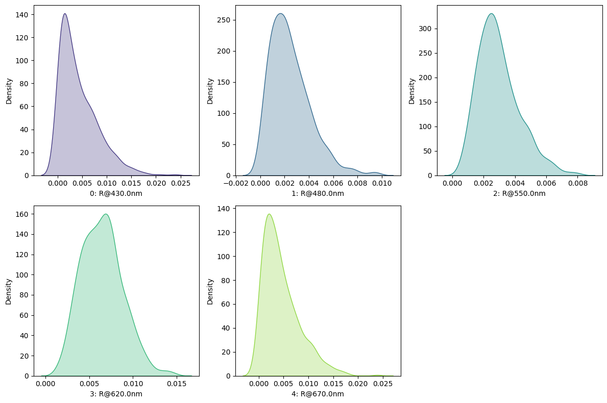
Read off yield from the CDF: e.g., what fraction of parts will have R < 1% at each wavelength?
fig, axes = mc.view_cdf()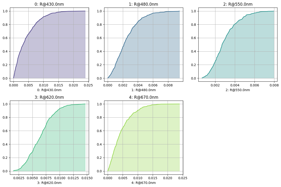
3c. Spectral tolerance band
This is the most informative plot: we compute the full reflectance spectrum for 200 random thickness perturbations. The shaded band shows the min/max envelope — the range of spectral performance you should expect in production.
# Store nominal thicknesses
nominal_thicknesses = [layer.thickness_um for layer in stack.layers]
rng = np.random.default_rng(42)

wl_band = np.linspace(400, 720, 200)
n_trials = 200
all_R = np.zeros((n_trials, len(wl_band)))

# Compute nominal spectrum on this grid
R_nom_band = np.array([ThinFilmOperand.reflectance(stack, wl) for wl in wl_band])

for trial in range(n_trials):
 # Apply random ±2% thickness perturbations to all layers
 for i, nom in enumerate(nominal_thicknesses):
     delta = rng.normal(0.0, 0.02)
     stack.layers[i].thickness_um = nom * (1.0 + delta)

 # Compute full spectrum
 all_R[trial] = [ThinFilmOperand.reflectance(stack, wl) for wl in wl_band]

 # Reset to nominal
 for i, nom in enumerate(nominal_thicknesses):
     stack.layers[i].thickness_um = nom

R_min = all_R.min(axis=0)
R_max = all_R.max(axis=0)
R_p05 = np.percentile(all_R, 5, axis=0)
R_p95 = np.percentile(all_R, 95, axis=0)

fig, ax = plt.subplots(figsize=(9, 5))
ax.fill_between(wl_band, R_min * 100, R_max * 100, alpha=0.15, color="steelblue",
             label="Min/max envelope")
ax.fill_between(wl_band, R_p05 * 100, R_p95 * 100, alpha=0.3, color="steelblue",
             label="5th–95th percentile")
ax.plot(wl_band, R_nom_band * 100, "-", color="darkblue", linewidth=2, label="Nominal")
ax.axhline(1.0, color="red", linestyle="--",
        linewidth=1, alpha=0.7, label="Spec: R < 1%")
ax.axvspan(420, 680, alpha=0.04, color="blue")
ax.set_xlabel("Wavelength (nm)")
ax.set_ylabel("Reflectance (%)")
ax.set_title("Spectral Tolerance Band — ±2% Thickness (7-Layer AR on N-BK7)")
ax.set_ylim(0, 4)
ax.legend(loc="upper right")
ax.grid(True, alpha=0.3)
fig.tight_layout();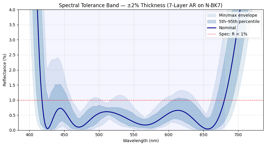
3d. Summary statistics and yield
df = mc.get_results()
operand_cols = [c for c in df.columns if "R@" in c]

print("Reflectance statistics under ±2% thickness tolerance (500 trials):\n")
print(df[operand_cols].describe().round(6))

# Yield analysis: fraction of parts meeting R < 1% at each wavelength
print("\nYield (fraction with R < 1%):")
for col in operand_cols:
 yield_pct = (df[col] < 0.01).mean() * 100
 print(f"  {col}: {yield_pct:.1f}%")
Show full code listing
import numpy as np
import matplotlib.pyplot as plt
from optiland.materials import Material, IdealMaterial
from optiland.thin_film import ThinFilmStack
from optiland.thin_film.optimization.operand.thin_film import ThinFilmOperand
from optiland.thin_film.tolerancing import (
  ThinFilmTolerancing,
  ThinFilmSensitivityAnalysis,
  ThinFilmMonteCarlo,
)
from optiland.tolerancing.perturbation import RangeSampler, DistributionSampler

air = IdealMaterial(n=1.0)
nbk7 = Material("N-BK7")
mgf2 = Material("MgF2", reference="Dodge-o")
al2o3 = Material("Al2O3", reference="Malitson")

# 7-layer design from needle synthesis (Tutorial 6h)
stack = ThinFilmStack(incident_material=air, substrate_material=nbk7)
stack.add_layer_nm(mgf2, 94.6, name="MgF2")
stack.add_layer_nm(al2o3, 319.7, name="Al2O3")
stack.add_layer_nm(mgf2, 17.7, name="MgF2")
stack.add_layer_nm(al2o3, 196.1, name="Al2O3")
stack.add_layer_nm(mgf2, 26.3, name="MgF2")
stack.add_layer_nm(al2o3, 170.9, name="Al2O3")
stack.add_layer_nm(mgf2, 190.4, name="MgF2")
print(stack)

wl_plot = np.linspace(400, 720, 300)
R_nominal = np.array([ThinFilmOperand.reflectance(stack, wl) for wl in wl_plot])

fig, ax = plt.subplots(figsize=(9, 5))
ax.plot(wl_plot, R_nominal * 100, "-", color="steelblue", linewidth=2, label="Nominal")
ax.axhline(1.0, color="red", linestyle="--",
         linewidth=1, alpha=0.7, label="Spec: R < 1%")
ax.axvspan(420, 680, alpha=0.06, color="blue", label="Target band")
ax.set_xlabel("Wavelength (nm)")
ax.set_ylabel("Reflectance (%)")
ax.set_title("Nominal Design — 7-Layer Broadband AR on N-BK7")
ax.set_ylim(0, 4)
ax.legend()
ax.grid(True, alpha=0.3)
fig.tight_layout();

tol = ThinFilmTolerancing(stack)

# Operands: reflectance at three key wavelengths
tol.add_operand("R", 450.0)
tol.add_operand("R", 550.0)
tol.add_operand("R", 650.0)

# ±3% thickness perturbation on each of the 7 layers
for i in range(7):
  tol.add_perturbation(i, "thickness", RangeSampler(-0.03, 0.03, 13))

sa = ThinFilmSensitivityAnalysis(tol)
sa.run()

fig, axes = sa.view()
fig.suptitle("Sensitivity: R vs. Layer Thickness Perturbation (±3%)", y=1.02)
fig.tight_layout();

# Identify which layers have the steepest sensitivity slopes
df_sa = sa.get_results()
operand_cols = [
  c for c in df_sa.columns
  if c.startswith("0:") or c.startswith("1:") or c.startswith("2:")
]

print("Sensitivity range (max - min reflectance) per layer:")
for ptype in df_sa["perturbation_type"].unique():
  mask = df_sa["perturbation_type"] == ptype
  ranges = df_sa.loc[mask, operand_cols].max() - df_sa.loc[mask, operand_cols].min()
  worst = ranges.max()
  print(f"  {ptype}: max ΔR = {worst*100:.3f}%")

tol_mc = ThinFilmTolerancing(stack)

# Operands: reflectance at 5 wavelengths across the band
for wl in [430.0, 480.0, 550.0, 620.0, 670.0]:
  tol_mc.add_operand("R", wl)

# 2% std thickness perturbation on all 7 layers
for i in range(7):
  tol_mc.add_perturbation(
      i, "thickness",
      DistributionSampler("normal", seed=100 + i, loc=0.0, scale=0.02),
  )

mc = ThinFilmMonteCarlo(tol_mc)
mc.run(num_iterations=500)
print(f"Monte Carlo complete: {len(mc.get_results())} trials")

fig, axes = mc.view_histogram(kde=True)

fig, axes = mc.view_cdf()

# Store nominal thicknesses
nominal_thicknesses = [layer.thickness_um for layer in stack.layers]
rng = np.random.default_rng(42)

wl_band = np.linspace(400, 720, 200)
n_trials = 200
all_R = np.zeros((n_trials, len(wl_band)))

# Compute nominal spectrum on this grid
R_nom_band = np.array([ThinFilmOperand.reflectance(stack, wl) for wl in wl_band])

for trial in range(n_trials):
  # Apply random ±2% thickness perturbations to all layers
  for i, nom in enumerate(nominal_thicknesses):
      delta = rng.normal(0.0, 0.02)
      stack.layers[i].thickness_um = nom * (1.0 + delta)

  # Compute full spectrum
  all_R[trial] = [ThinFilmOperand.reflectance(stack, wl) for wl in wl_band]

  # Reset to nominal
  for i, nom in enumerate(nominal_thicknesses):
      stack.layers[i].thickness_um = nom

R_min = all_R.min(axis=0)
R_max = all_R.max(axis=0)
R_p05 = np.percentile(all_R, 5, axis=0)
R_p95 = np.percentile(all_R, 95, axis=0)

fig, ax = plt.subplots(figsize=(9, 5))
ax.fill_between(wl_band, R_min * 100, R_max * 100, alpha=0.15, color="steelblue",
              label="Min/max envelope")
ax.fill_between(wl_band, R_p05 * 100, R_p95 * 100, alpha=0.3, color="steelblue",
              label="5th–95th percentile")
ax.plot(wl_band, R_nom_band * 100, "-", color="darkblue", linewidth=2, label="Nominal")
ax.axhline(1.0, color="red", linestyle="--",
         linewidth=1, alpha=0.7, label="Spec: R < 1%")
ax.axvspan(420, 680, alpha=0.04, color="blue")
ax.set_xlabel("Wavelength (nm)")
ax.set_ylabel("Reflectance (%)")
ax.set_title("Spectral Tolerance Band — ±2% Thickness (7-Layer AR on N-BK7)")
ax.set_ylim(0, 4)
ax.legend(loc="upper right")
ax.grid(True, alpha=0.3)
fig.tight_layout();

df = mc.get_results()
operand_cols = [c for c in df.columns if "R@" in c]

print("Reflectance statistics under ±2% thickness tolerance (500 trials):\n")
print(df[operand_cols].describe().round(6))

# Yield analysis: fraction of parts meeting R < 1% at each wavelength
print("\nYield (fraction with R < 1%):")
for col in operand_cols:
  yield_pct = (df[col] < 0.01).mean() * 100
  print(f"  {col}: {yield_pct:.1f}%")
Conclusions
Interpretation
- The sensitivity analysis reveals which layers dominate the error budget — steep curves mean tight thickness control is needed on that layer.
- The spectral tolerance band shows the full range of reflectance spectra under manufacturing variations. Where the max envelope crosses the 1% spec line indicates the wavelengths most at risk.
- The yield analysis quantifies what fraction of manufactured parts will meet spec at each wavelength — this directly informs go/no-go decisions for production tolerances.
- For this 7-layer AR coating, ±2% thickness control (achievable with modern ion-beam sputtering) keeps reflectance well within spec across most of the band.
Next tutorials
Original notebook: Tutorial_6i_Thin_Film_Tolerance_Analysis.ipynb on GitHub · ReadTheDocs