Surface Roughness & Scattering
Model stray light and haze caused by micro-scale surface imperfections.
Introduction
This tutorial demonstrates how surface roughness and scattering can be configured on surfaces in Optiland. We will compare singlets with the following scattering properties assigned:
- No scattering
- Gaussian Scattering
- Lambertian Scattering
The scattering model is defined via the Bidirectional Scattering Distribution Function, or BSDF.
Core concepts used
Step-by-step build
Import Libraries
import matplotlib.pyplot as plt
 import numpy as np

from optiland import optic, scatterDefine Configurable Singlet Class
Preparation
We first define a generic singlet class that accepts a bsdf as an input. In this example, we assign the scattering only to the rear surface.
class SingletConfigurable(optic.Optic):
 def __init__(self, bsdf):
     super().__init__()

     # add surfaces
     self.add_surface(index=0, radius=np.inf, thickness=np.inf)
     self.add_surface(
         index=1,
         thickness=7,
         radius=50,
         is_stop=True,
         material="N-SF11",
     )
     self.add_surface(index=2, thickness=50, bsdf=bsdf)  # <-- add bsdf here
     self.add_surface(index=3)

     # add aperture
     self.set_aperture(aperture_type="EPD", value=25.4)

     # add field
     self.set_field_type(field_type="angle")
     self.add_field(y=0)
     self.add_field(y=10)
     self.add_field(y=14)

     # add wavelength
     self.add_wavelength(value=0.48613270)
     self.add_wavelength(value=0.58756180, is_primary=True)
     self.add_wavelength(value=0.65627250)

self.image_solve() # solve for image planeAdd Ray Distribution Helper
Let's also define a helper function to plot a 2D distribution of rays intersection points.
def plot_ray_distribution(rays, bins=128):
 x = rays.x
 y = rays.y
 i = rays.i

 plt.hist2d(x, y, weights=i, bins=bins, cmap="viridis")
 plt.colorbar()
 plt.xlabel("X (mm)")
 plt.ylabel("Y (mm)")
 plt.title("2D Ray Distribution on Image Plane")
plt.show()Build Singlet Without Scattering
The first singlet we analyze will have no scattering applied. Let's first define the lens and draw it.
singlet_no_scatter = SingletConfigurable(bsdf=None)Draw the Unscattered Singlet
singlet_no_scatter.draw()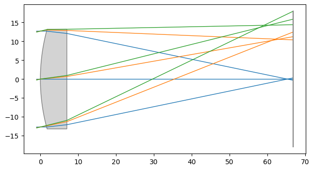
Trace 1M Rays and Plot Distribution
Let's trace 1 million random rays through the lens at the on-axis field point and look at the distribution.
rays = singlet_no_scatter.trace(
 Hx=0,
 Hy=0,
 wavelength=0.58756180,
 num_rays=1_000_000,
 distribution="random",
)

plot_ray_distribution(rays, bins=128)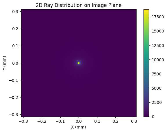
Apply Gaussian BSDF Scattering
As we can see, the energy is largely located at the origin on the image plane. Let's see how this is implacted when scattering is introduced.
Gaussian scattering is defined by a 2D Gaussian distribution with a user-defined sigma (std. dev.) value. The larger the value of sigma, the closer the scattering model comes to Lambertian. We define a GaussianBSDF model with a sigma value of 0.01 and generate a new singlet:
bsdf = scatter.GaussianBSDF(sigma=0.01)
singlet_gaussian = SingletConfigurable(bsdf=bsdf)Trace Rays Through Gaussian Singlet
Again, we trace 1 million rays and view the distribution at the image plane:
rays = singlet_gaussian.trace(
 Hx=0,
 Hy=0,
 wavelength=0.58756180,
 num_rays=1_000_000,
 distribution="random",
)

plot_ray_distribution(rays)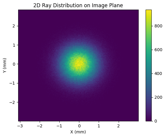
Apply Lambertian BSDF Scattering
The image size has blurred significantly in comparison to the no-scattering case. Note that the plot axis spans a larger range here as well.
Lambertian scattering implies that the surface scatters incident light uniformly in all directions. Diffuse surfaces can be considered approximately Lambertian. To model a Lambertian scatterer in Optiland, we simply define the LambertianBSDF model and pass it to our singlet:
bsdf = scatter.LambertianBSDF()
singlet_lambertian = SingletConfigurable(bsdf=bsdf)Trace Rays Through Lambertian Singlet
rays = singlet_lambertian.trace(
 Hx=0,
 Hy=0,
 wavelength=0.58756180,
 num_rays=1_000_000,
 distribution="random",
)

plot_ray_distribution(rays, bins=np.linspace(-100, 100, 128))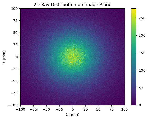
Show full code listing
import matplotlib.pyplot as plt
import numpy as np

from optiland import optic, scatter

class SingletConfigurable(optic.Optic):
  def __init__(self, bsdf):
      super().__init__()

      # add surfaces
      self.add_surface(index=0, radius=np.inf, thickness=np.inf)
      self.add_surface(
          index=1,
          thickness=7,
          radius=50,
          is_stop=True,
          material="N-SF11",
      )
      self.add_surface(index=2, thickness=50, bsdf=bsdf)  # <-- add bsdf here
      self.add_surface(index=3)

      # add aperture
      self.set_aperture(aperture_type="EPD", value=25.4)

      # add field
      self.set_field_type(field_type="angle")
      self.add_field(y=0)
      self.add_field(y=10)
      self.add_field(y=14)

      # add wavelength
      self.add_wavelength(value=0.48613270)
      self.add_wavelength(value=0.58756180, is_primary=True)
      self.add_wavelength(value=0.65627250)

      self.image_solve()  # solve for image plane

def plot_ray_distribution(rays, bins=128):
  x = rays.x
  y = rays.y
  i = rays.i

  plt.hist2d(x, y, weights=i, bins=bins, cmap="viridis")
  plt.colorbar()
  plt.xlabel("X (mm)")
  plt.ylabel("Y (mm)")
  plt.title("2D Ray Distribution on Image Plane")
  plt.show()

singlet_no_scatter = SingletConfigurable(bsdf=None)

singlet_no_scatter.draw()

rays = singlet_no_scatter.trace(
  Hx=0,
  Hy=0,
  wavelength=0.58756180,
  num_rays=1_000_000,
  distribution="random",
)

plot_ray_distribution(rays, bins=128)

bsdf = scatter.GaussianBSDF(sigma=0.01)
singlet_gaussian = SingletConfigurable(bsdf=bsdf)

rays = singlet_gaussian.trace(
  Hx=0,
  Hy=0,
  wavelength=0.58756180,
  num_rays=1_000_000,
  distribution="random",
)

plot_ray_distribution(rays)

bsdf = scatter.LambertianBSDF()
singlet_lambertian = SingletConfigurable(bsdf=bsdf)

rays = singlet_lambertian.trace(
  Hx=0,
  Hy=0,
  wavelength=0.58756180,
  num_rays=1_000_000,
  distribution="random",
)

plot_ray_distribution(rays, bins=np.linspace(-100, 100, 128))
Conclusions
In this case, we are plotting the image plane over a significantly larger area, from -100 mm to 100 mm. Clearly, the Lambertian scatter model has dramatically increased the spot size at the image plane.
- Conclusions:
- We introduced two BSDF scatter models: Gaussian and Lambertian.
- Scatter models can be used to model and understand the impact of manufacturing defects, such as surface roughness on optical surfaces.
Next tutorials
Original notebook: Tutorial_7b_Surface_Roughness_%26_Scattering.ipynb on GitHub · ReadTheDocs