Advanced Design

Freeform Surfaces

Break symmetry with high-order polynomial surfaces for complex beam shaping.

AdvancedAdvanced Optical DesignNumPy backend12 min read

Introduction

This tutorial demonstrates how freeform surfaces can be modeled in Optiland. Several freeform types are supported, including polynomial and Chebyshev surfaces.

In this tutorial, we will design a unique singlet lens with the following properties:

rays from on-axis field point intersect the image plane at y=3mm
RMS spot size is minimized

This is rather unique (and perhaps not all that useful), as rays from the on-axis field point in a standard lens are generally centered on the optical axis.

Core concepts used

surface_type='polynomial'

Defines a surface where the sag

z

is a combination of a traditional conic and an XY-polynomial expansion.

problem.add_variable(..., 'polynomial_coeff')

Allows the optimizer to adjust individual coefficients of the XY-polynomial (e.g.,

x^1, y^1, x^2, \dots

coeff_index=(i, j)

Specifies exactly which term of the

C_{i,j} \cdot x^i y^j

expansion to vary.

real_y_intercept

Used here as a 'steering' target to force rays to a specific coordinate off the optical axis.

Step-by-step build

Import Libraries

python

import numpy as np

from optiland import analysis, optic, optimization

Define Freeform Polynomial Lens Class

Preparation:

We start by defining a freeform lens class, which has a freeform as its first surface.

The freeform surface is defined as:

z(x, y) = \frac{r^2}{R\left(1 + \sqrt{1 - (1 + k)\, \frac{r^2}{R^2}}\right)} + \sum_i \sum_j C_{i,j}\, x^i y^j

where

$x$ and $y$ are the local surface coordinates
$r^2 = x^2 + y^2$
$R$ is the radius of curvature
$k$ is the conic constant

$C_{i,j}$ is the polynomial coefficient for indices $i, j$

python

class Freeform(optic.Optic):
 def __init__(self):
     super().__init__()

     # add surfaces
     self.add_surface(index=0, radius=np.inf, thickness=np.inf)

     # ======== Add polynomial freeform here =====================================
     self.add_surface(
         index=1,
         radius=100,
         thickness=5,
         surface_type="polynomial",  # <-- surface_type='polynomial'
         is_stop=True,
         material="SF11",
         coefficients=[],
     )
     # ===========================================================================

     self.add_surface(index=2, thickness=100)
     self.add_surface(index=3)

     # add aperture
     self.set_aperture(aperture_type="EPD", value=25)

     # add field
     self.set_field_type(field_type="angle")
     self.add_field(y=0)

     # add wavelength
     self.add_wavelength(value=0.55, is_primary=True)

Draw the Starting-Point Lens

We simply need to specify the surface type as 'polynomial' to make the first surface a freeform. Note that we did not pass coefficients to the surface, which implies all coefficients will be zero.

Let's generate and view the starting point lens, which will simply be spherical, as the freeform coefficients are all zero.

python

lens = Freeform()
lens.draw(num_rays=5)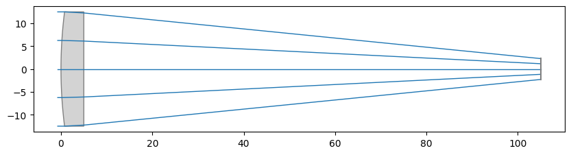

Set Up Optimization Operands

We now define the optimization problem. Let's start with the two operands: 1) RMS spot size and 2) real ray y-intercept.

python

problem = optimization.OptimizationProblem()

# RMS spot size operand
input_data = {
 "optic": lens,
 "surface_number": -1,
 "Hx": 0,
 "Hy": 0,
 "wavelength": 0.55,
 "num_rays": 5,
}
problem.add_operand(
 operand_type="rms_spot_size",
 target=0,
 weight=1,
 input_data=input_data,
)

# Real y-intercept operand
input_data = {
 "optic": lens,
 "surface_number": -1,
 "Hx": 0,
 "Hy": 0,
 "Px": 0,
 "Py": 0,
 "wavelength": 0.55,
}
problem.add_operand(
 operand_type="real_y_intercept",
 target=3,
 weight=1,
 input_data=input_data,
)  # <-- target=3

Add Polynomial Coefficients as Variables

We will include the first 9 polynomial coefficients of our surface as variables. We will not add bounds for the coefficients.

python

for i in range(3):
 for j in range(3):
     problem.add_variable(
         lens,
         "polynomial_coeff",
         surface_number=1,
         coeff_index=(i, j),
     )

problem.info()

Run the Optimizer

Let's optimize and observe the merit function improvement.

python

optimizer = optimization.OptimizerGeneric(problem)
res = optimizer.optimize(tol=1e-9)

Inspect Post-Optimization Merit Function

python

problem.info()

Draw the Optimized Freeform Lens

Finally, we plot the lens and view a spot diagram.

python

lens.draw(num_rays=5)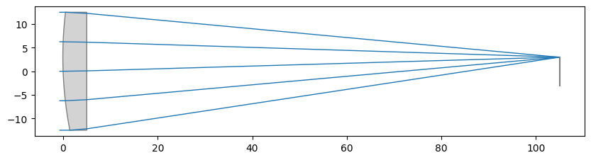

View the Spot Diagram

python

spot = analysis.SpotDiagram(lens)
spot.view()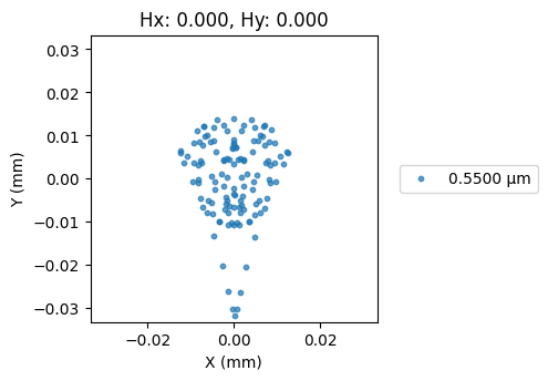

Show full code listing

python

import numpy as np

from optiland import analysis, optic, optimization

class Freeform(optic.Optic):
  def __init__(self):
      super().__init__()

      # add surfaces
      self.add_surface(index=0, radius=np.inf, thickness=np.inf)

      # ======== Add polynomial freeform here =====================================
      self.add_surface(
          index=1,
          radius=100,
          thickness=5,
          surface_type="polynomial",  # <-- surface_type='polynomial'
          is_stop=True,
          material="SF11",
          coefficients=[],
      )
      # ===========================================================================

      self.add_surface(index=2, thickness=100)
      self.add_surface(index=3)

      # add aperture
      self.set_aperture(aperture_type="EPD", value=25)

      # add field
      self.set_field_type(field_type="angle")
      self.add_field(y=0)

      # add wavelength
      self.add_wavelength(value=0.55, is_primary=True)

lens = Freeform()
lens.draw(num_rays=5)

problem = optimization.OptimizationProblem()

# RMS spot size operand
input_data = {
  "optic": lens,
  "surface_number": -1,
  "Hx": 0,
  "Hy": 0,
  "wavelength": 0.55,
  "num_rays": 5,
}
problem.add_operand(
  operand_type="rms_spot_size",
  target=0,
  weight=1,
  input_data=input_data,
)

# Real y-intercept operand
input_data = {
  "optic": lens,
  "surface_number": -1,
  "Hx": 0,
  "Hy": 0,
  "Px": 0,
  "Py": 0,
  "wavelength": 0.55,
}
problem.add_operand(
  operand_type="real_y_intercept",
  target=3,
  weight=1,
  input_data=input_data,
)  # <-- target=3

for i in range(3):
  for j in range(3):
      problem.add_variable(
          lens,
          "polynomial_coeff",
          surface_number=1,
          coeff_index=(i, j),
      )

problem.info()

optimizer = optimization.OptimizerGeneric(problem)
res = optimizer.optimize(tol=1e-9)

problem.info()

lens.draw(num_rays=5)

spot = analysis.SpotDiagram(lens)
spot.view()

Conclusions

We clearly see that the front surface of our lens appears to be tilted, which forces the on-axis rays to intercept the image plane near y=3mm.

Conclusions:

We introduced freeform surfaces in Optiland.
We optimized a singlet lens for minimal spot size and for an off-axis real ray intercept point.
Additional freeform surfaces are available and can be found in the optiland.geometries module or the documentation.

Next tutorials

NextThree-Mirror AnastigmatImplement a classic all-reflective freeform telescope design.RelatedSurface Roughness & ScatteringUnderstand how manufacturing errors on these freeform surfaces cause stray light.

Original notebook: Tutorial_7c_Freeform_Surfaces.ipynb on GitHub · ReadTheDocs