Advanced Design
Three-Mirror Anastigmat
Implement a classic all-reflective freeform telescope design.
AdvancedAdvanced Optical DesignNumPy backend15 min read
Introduction
This tutorial aims at demonstrating Optiland's capabilities in reflective systems design using freeform mirrors.
Setup the telescope
The starting telescope is voluntarily defocused, it will be optimized after.
Core concepts used
material='mirror'
Tells Optiland to reflect rays at the interface rather than refract them.
surface_type='zernike'
Uses Zernike polynomials to add non-rotationally symmetric 'figure' to the mirrors, correcting off-axis coma and astigmatism.
real_y_intercept_lcs
A specialized operand that targets ray coordinates in the surface's local tilted/decentered frame rather than the global frame.
rx=np.radians(-15.0)
Applies a mechanical tilt (in radians) to the surface around the X-axis.
Step-by-step build
1
Import NumPy and Optiland modules
python
import numpy as np
from optiland import analysis, optic, optimization
focal_length = 100 # [mm]
lens = optic.Optic(name="TMA")
lens.set_aperture(aperture_type="EPD", value=10)
lens.set_field_type(field_type="angle")
lens.add_field(y=0)
lens.add_field(y=+1.5)
lens.add_field(y=-1.5)
lens.add_wavelength(value=0.486)
lens.add_wavelength(value=0.587, is_primary=True)
lens.add_wavelength(value=0.656)
# The telescope is made of three freeform surfaces (Zernike)
lens.add_surface(index=0, radius=np.inf, thickness=np.inf)
lens.add_surface(
index=1,
radius=-100,
thickness=-20,
conic=0,
material="mirror",
rx=np.radians(-15.0),
is_stop=True,
surface_type="zernike",
coefficients=[],
)
lens.add_surface(
index=2,
radius=-100,
thickness=+20,
conic=0,
material="mirror",
rx=np.radians(-10.0),
dy=-11.5,
surface_type="zernike",
coefficients=[],
)
lens.add_surface(
index=3,
radius=-100,
thickness=-22,
conic=0,
material="mirror",
rx=np.radians(-1.0),
dy=-15,
surface_type="zernike",
coefficients=[],
)
lens.add_surface(index=4, dy=-19.3)
lens.update_paraxial()
lens.draw(title=lens.name)
lens.info()
# lens.draw3D()
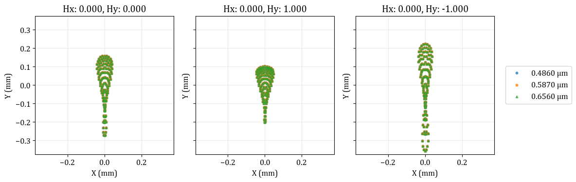
spot = analysis.SpotDiagram(lens)
spot.view()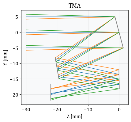
2
Optimization
The optimization variables are the radii, thicknesses, decenters & tilts, and the freeform coefficients.
We define contraints on the mirrors' decenters to prevent vignetting.
Variables
python
problem = optimization.OptimizationProblem()

# radii
problem.add_variable(lens, "radius", surface_number=1, min_val=-1000, max_val=1000)
problem.add_variable(lens, "radius", surface_number=2, min_val=-1000, max_val=1000)
problem.add_variable(lens, "radius", surface_number=3, min_val=-1000, max_val=1000)

# thicknesses
problem.add_variable(lens, "thickness", surface_number=1, min_val=-35, max_val=-15)
problem.add_variable(lens, "thickness", surface_number=2, min_val=+15, max_val=+35)
problem.add_variable(lens, "thickness", surface_number=3, min_val=-35, max_val=-15)

# decenters
problem.add_variable(
 lens,
 "decenter",
 axis="y",
 surface_number=2,
 min_val=-15,
 max_val=-10,
)
problem.add_variable(
 lens,
 "decenter",
 axis="y",
 surface_number=3,
 min_val=-20,
 max_val=-11,
)
problem.add_variable(
 lens,
 "decenter",
 axis="y",
 surface_number=4,
 min_val=-28,
 max_val=-22,
)

# tilts
problem.add_variable(
 lens,
 "tilt",
 axis="x",
 surface_number=1,
 min_val=np.radians(-20.0),
 max_val=np.radians(-12.0),
)
problem.add_variable(
 lens,
 "tilt",
 axis="x",
 surface_number=2,
 min_val=np.radians(-15.0),
 max_val=np.radians(-08.0),
)
problem.add_variable(
 lens,
 "tilt",
 axis="x",
 surface_number=3,
 min_val=np.radians(-10.0),
 max_val=np.radians(+10.0),
)

# conic constants
problem.add_variable(lens, "conic", surface_number=1, min_val=-10, max_val=10)
problem.add_variable(lens, "conic", surface_number=2, min_val=-10, max_val=10)
problem.add_variable(lens, "conic", surface_number=3, min_val=-10, max_val=10)

# Freeform coefficients
for s in range(1, 4):
 for i in range(4):
     problem.add_variable(
         lens,
         "zernike_coeff",
         surface_number=s,
         coeff_index=i,
         min_val=-1,
         max_val=1,
     )
3
Operands
python
# Center M2 on its chief ray
input_data = {
 "optic": lens,
 "surface_number": 2,
 "Hx": 0,
 "Hy": 0,
 "Px": 0,
 "Py": 0,
 "wavelength": lens.wavelengths.primary_wavelength.value,
}
problem.add_operand(
 operand_type="real_y_intercept_lcs",
 target=0.0,
 weight=1,
 input_data=input_data,
)

# Center M3 on its chief ray
input_data = {
 "optic": lens,
 "surface_number": 3,
 "Hx": 0,
 "Hy": 0,
 "Px": 0,
 "Py": 0,
 "wavelength": lens.wavelengths.primary_wavelength.value,
}
problem.add_operand(
 operand_type="real_y_intercept_lcs",
 target=0.0,
 weight=1,
 input_data=input_data,
)

# Image surface - Real ray heights operands, in the lcs of the image surface
# Center the image surface on its chief ray
input_data = {
 "optic": lens,
 "surface_number": 4,
 "Hx": 0,
 "Hy": 0,
 "Px": 0,
 "Py": 0,
 "wavelength": lens.wavelengths.primary_wavelength.value,
}
problem.add_operand(
 operand_type="real_y_intercept_lcs",
 target=focal_length * np.tan(np.deg2rad(lens.fields.y_fields[0])),
 weight=1,
 input_data=input_data,
)
input_data = {
 "optic": lens,
 "surface_number": 4,
 "Hx": 0,
 "Hy": 1,
 "Px": 0,
 "Py": 0,
 "wavelength": lens.wavelengths.primary_wavelength.value,
}
problem.add_operand(
 operand_type="real_y_intercept_lcs",
 target=focal_length * np.tan(np.deg2rad(lens.fields.y_fields[1])),
 weight=1,
 input_data=input_data,
)
input_data = {
 "optic": lens,
 "surface_number": 4,
 "Hx": 0,
 "Hy": -1,
 "Px": 0,
 "Py": 0,
 "wavelength": lens.wavelengths.primary_wavelength.value,
}
problem.add_operand(
 operand_type="real_y_intercept_lcs",
 target=focal_length * np.tan(np.deg2rad(lens.fields.y_fields[2])),
 weight=1,
 input_data=input_data,
)

# RMS spot size: minimize the spot size for each field at the primary wavelength.
# We choose a 'uniform' distribution, so the number of rays actually means the rays on
# one axis. Therefore we trace ≈16^2 rays here.
for field in lens.fields.get_field_coords():
 input_data = {
     "optic": lens,
     "surface_number": 4,
     "Hx": field[0],
     "Hy": field[1],
     "num_rays": 16,
     "wavelength": 0.587,
     "distribution": "uniform",
 }
 problem.add_operand(
     operand_type="rms_spot_size",
     target=0.0,
     weight=10,
     input_data=input_data,
 )

problem.info()
4
Optimization
python
# Local optimizer
optimizer = optimization.OptimizerGeneric(problem)
res = optimizer.optimize(tol=1e-9)

# Global optimizer
# optimizer = optimization.DifferentialEvolution(problem)
# res = optimizer.optimize(maxiter=100, workers=-1)

lens.info()
lens.draw(title=f"Optimized {lens.name}")
problem.info()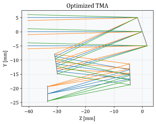
5
Inspect the optimized spot diagram
python
spot = analysis.SpotDiagram(lens)
spot.view()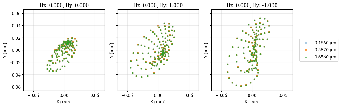
6
Plot the geometric MTF
python
from optiland.mtf import GeometricMTF

geo_mtf = GeometricMTF(lens)
geo_mtf.view()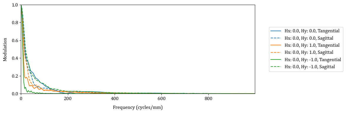
Show full code listing
python
import numpy as np

from optiland import analysis, optic, optimization

focal_length = 100  # [mm]

lens = optic.Optic(name="TMA")
lens.set_aperture(aperture_type="EPD", value=10)
lens.set_field_type(field_type="angle")
lens.add_field(y=0)
lens.add_field(y=+1.5)
lens.add_field(y=-1.5)
lens.add_wavelength(value=0.486)
lens.add_wavelength(value=0.587, is_primary=True)
lens.add_wavelength(value=0.656)

# The telescope is made of three freeform surfaces (Zernike)
lens.add_surface(index=0, radius=np.inf, thickness=np.inf)
lens.add_surface(
  index=1,
  radius=-100,
  thickness=-20,
  conic=0,
  material="mirror",
  rx=np.radians(-15.0),
  is_stop=True,
  surface_type="zernike",
  coefficients=[],
)
lens.add_surface(
  index=2,
  radius=-100,
  thickness=+20,
  conic=0,
  material="mirror",
  rx=np.radians(-10.0),
  dy=-11.5,
  surface_type="zernike",
  coefficients=[],
)
lens.add_surface(
  index=3,
  radius=-100,
  thickness=-22,
  conic=0,
  material="mirror",
  rx=np.radians(-1.0),
  dy=-15,
  surface_type="zernike",
  coefficients=[],
)
lens.add_surface(index=4, dy=-19.3)

lens.update_paraxial()
lens.draw(title=lens.name)
lens.info()
# lens.draw3D()
spot = analysis.SpotDiagram(lens)
spot.view()

problem = optimization.OptimizationProblem()

# radii
problem.add_variable(lens, "radius", surface_number=1, min_val=-1000, max_val=1000)
problem.add_variable(lens, "radius", surface_number=2, min_val=-1000, max_val=1000)
problem.add_variable(lens, "radius", surface_number=3, min_val=-1000, max_val=1000)

# thicknesses
problem.add_variable(lens, "thickness", surface_number=1, min_val=-35, max_val=-15)
problem.add_variable(lens, "thickness", surface_number=2, min_val=+15, max_val=+35)
problem.add_variable(lens, "thickness", surface_number=3, min_val=-35, max_val=-15)

# decenters
problem.add_variable(
  lens,
  "decenter",
  axis="y",
  surface_number=2,
  min_val=-15,
  max_val=-10,
)
problem.add_variable(
  lens,
  "decenter",
  axis="y",
  surface_number=3,
  min_val=-20,
  max_val=-11,
)
problem.add_variable(
  lens,
  "decenter",
  axis="y",
  surface_number=4,
  min_val=-28,
  max_val=-22,
)

# tilts
problem.add_variable(
  lens,
  "tilt",
  axis="x",
  surface_number=1,
  min_val=np.radians(-20.0),
  max_val=np.radians(-12.0),
)
problem.add_variable(
  lens,
  "tilt",
  axis="x",
  surface_number=2,
  min_val=np.radians(-15.0),
  max_val=np.radians(-08.0),
)
problem.add_variable(
  lens,
  "tilt",
  axis="x",
  surface_number=3,
  min_val=np.radians(-10.0),
  max_val=np.radians(+10.0),
)

# conic constants
problem.add_variable(lens, "conic", surface_number=1, min_val=-10, max_val=10)
problem.add_variable(lens, "conic", surface_number=2, min_val=-10, max_val=10)
problem.add_variable(lens, "conic", surface_number=3, min_val=-10, max_val=10)

# Freeform coefficients
for s in range(1, 4):
  for i in range(4):
      problem.add_variable(
          lens,
          "zernike_coeff",
          surface_number=s,
          coeff_index=i,
          min_val=-1,
          max_val=1,
      )

# Center M2 on its chief ray
input_data = {
  "optic": lens,
  "surface_number": 2,
  "Hx": 0,
  "Hy": 0,
  "Px": 0,
  "Py": 0,
  "wavelength": lens.wavelengths.primary_wavelength.value,
}
problem.add_operand(
  operand_type="real_y_intercept_lcs",
  target=0.0,
  weight=1,
  input_data=input_data,
)

# Center M3 on its chief ray
input_data = {
  "optic": lens,
  "surface_number": 3,
  "Hx": 0,
  "Hy": 0,
  "Px": 0,
  "Py": 0,
  "wavelength": lens.wavelengths.primary_wavelength.value,
}
problem.add_operand(
  operand_type="real_y_intercept_lcs",
  target=0.0,
  weight=1,
  input_data=input_data,
)

# Image surface - Real ray heights operands, in the lcs of the image surface
# Center the image surface on its chief ray
input_data = {
  "optic": lens,
  "surface_number": 4,
  "Hx": 0,
  "Hy": 0,
  "Px": 0,
  "Py": 0,
  "wavelength": lens.wavelengths.primary_wavelength.value,
}
problem.add_operand(
  operand_type="real_y_intercept_lcs",
  target=focal_length * np.tan(np.deg2rad(lens.fields.y_fields[0])),
  weight=1,
  input_data=input_data,
)
input_data = {
  "optic": lens,
  "surface_number": 4,
  "Hx": 0,
  "Hy": 1,
  "Px": 0,
  "Py": 0,
  "wavelength": lens.wavelengths.primary_wavelength.value,
}
problem.add_operand(
  operand_type="real_y_intercept_lcs",
  target=focal_length * np.tan(np.deg2rad(lens.fields.y_fields[1])),
  weight=1,
  input_data=input_data,
)
input_data = {
  "optic": lens,
  "surface_number": 4,
  "Hx": 0,
  "Hy": -1,
  "Px": 0,
  "Py": 0,
  "wavelength": lens.wavelengths.primary_wavelength.value,
}
problem.add_operand(
  operand_type="real_y_intercept_lcs",
  target=focal_length * np.tan(np.deg2rad(lens.fields.y_fields[2])),
  weight=1,
  input_data=input_data,
)

# RMS spot size: minimize the spot size for each field at the primary wavelength.
# We choose a 'uniform' distribution, so the number of rays actually means the rays on
# one axis. Therefore we trace ≈16^2 rays here.
for field in lens.fields.get_field_coords():
  input_data = {
      "optic": lens,
      "surface_number": 4,
      "Hx": field[0],
      "Hy": field[1],
      "num_rays": 16,
      "wavelength": 0.587,
      "distribution": "uniform",
  }
  problem.add_operand(
      operand_type="rms_spot_size",
      target=0.0,
      weight=10,
      input_data=input_data,
  )

problem.info()

# Local optimizer
optimizer = optimization.OptimizerGeneric(problem)
res = optimizer.optimize(tol=1e-9)

# Global optimizer
# optimizer = optimization.DifferentialEvolution(problem)
# res = optimizer.optimize(maxiter=100, workers=-1)

lens.info()
lens.draw(title=f"Optimized {lens.name}")
problem.info()

spot = analysis.SpotDiagram(lens)
spot.view()

from optiland.mtf import GeometricMTF

geo_mtf = GeometricMTF(lens)
geo_mtf.view()
Conclusions
- A three-mirror anastigmat (TMA) telescope was constructed using three tilted and decentered freeform (Zernike) mirror surfaces, demonstrating Optiland's support for all-reflective, off-axis optical systems.
- The optimization problem included a rich set of variables — mirror radii, thicknesses, tilts, decenters, conic constants, and Zernike polynomial coefficients — showing how to handle highly parameterized freeform designs.
- The
real_y_intercept_lcsoperand was used to center each mirror and the image surface on their respective chief rays in the local coordinate frame, a technique that is essential for unobscured reflective geometries. - After optimization, the spot diagram showed a dramatic reduction in aberrations across all three field angles, confirming that the freeform coefficients effectively corrected off-axis coma and astigmatism.
- The geometric MTF plot provided a final, quantitative assessment of image quality, completing a full design-to-verification workflow for an advanced reflective system.
Next tutorials
NextStray Light AnalysisAnalyze unwanted reflections and 'ghosts' in complex reflective systems.RelatedFreeform SurfacesA foundational look at the polynomial surfaces used in this TMA design.
Original notebook: Tutorial_7d_Three_Mirror_Anastigmat.ipynb on GitHub · ReadTheDocs