Advanced Design
Glass Expert
Let the optimizer automatically select the best glass types from commercial catalogs.
AdvancedAdvanced Optical DesignNumPy backend15 min read
Introduction
This tutorial aims at demonstrating Optiland's capabilities in performing optimization on glass materials, in order to suggest a good combination to the user.
A description of GlassExpert's architecture can be found in the documentation (Developer's Guide: Categorical Optimization with Glass Expert)
Core concepts used
optimization.GlassExpert(problem)
A specialized optimizer designed for 'categorical' variables. It can handle discrete choices (like glass names) alongside continuous ones (like lens thickness).
glasses_selection(catalogs=['schott', 'ohara'])
Filters and prepares a subset of the material database for the optimizer to choose from.
problem.add_variable(..., 'material')
Flags a lens element as 'mutable,' allowing the optimizer to swap its material entirely during the search.
Step-by-step build
1
Import the backend, optic, and optimization modules
python
import optiland.backend as be
from optiland import optic, optimization
from optiland.materials import glasses_selection

target_focal_length = 100  # [mm]


class SixLensesStartPoint(optic.Optic):
 """A 6 lens design with very poor quality meant to be optimized."""

 def __init__(self):
     super().__init__()

     self.add_surface(index=0, radius=be.inf, thickness=be.inf)
     self.add_surface(index=1, radius=1000, thickness=25, material="N-BK7")
     self.add_surface(index=2, radius=1000, thickness=5.0)
     self.add_surface(index=3, radius=1000, thickness=25, material="N-BK7")
     self.add_surface(index=4, radius=be.inf, thickness=25, material="N-BK7")
     self.add_surface(index=5, radius=1000, thickness=25)
     self.add_surface(index=6, radius=be.inf, thickness=25.0, is_stop=True)
     self.add_surface(index=7, radius=-1000, thickness=25, material="N-BK7")
     self.add_surface(index=8, radius=be.inf, thickness=25, material="N-BK7")
     self.add_surface(index=9, radius=-1000, thickness=5.0)
     self.add_surface(index=10, radius=1000, thickness=25, material="N-BK7")
     self.add_surface(index=11, radius=-1000, thickness=200)
     self.add_surface(index=12)

     self.set_aperture(aperture_type="imageFNO", value=5)
     self.set_field_type(field_type="angle")

     self.add_field(y=-14)
     self.add_field(y=-10)
     self.add_field(y=0)
     self.add_field(y=10)
     self.add_field(y=14)

     self.add_wavelength(value=0.4861)
     self.add_wavelength(value=0.5876, is_primary=True)
     self.add_wavelength(value=0.6563)


lens = SixLensesStartPoint()
lens.draw(title="Starting lens")
lens.info()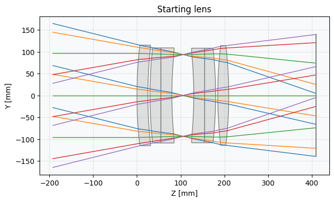
2
Operands
python
problem = optimization.OptimizationProblem()

# Real ray height to define the focal length
for k, hy in enumerate([-1, -0.714, 0, 0.714, 1]):
 input_data = {
     "optic": lens,
     "surface_number": 12,
     "Hx": 0,
     "Hy": hy,
     "Px": 0,
     "Py": 0,
     "wavelength": lens.wavelengths.primary_wavelength.value,
 }
 problem.add_operand(
     operand_type="real_y_intercept_lcs",
     target=target_focal_length * be.tan(be.deg2rad(lens.fields.y_fields[k])),
     weight=1,
     input_data=input_data,
 )

# RMS spot size - Minimize the spot size for each field at the primary wavelength.
# We choose a 'uniform' distribution, so the number of rays actually means the rays on
# one axis. Therefore we trace ≈16^2 rays here.
for field in lens.fields.get_field_coords():
 input_data = {
     "optic": lens,
     "surface_number": 12,
     "Hx": field[0],
     "Hy": field[1],
     "num_rays": 16,
     "wavelength": lens.wavelengths.primary_wavelength.value,
     "distribution": "uniform",
 }
 problem.add_operand(
     operand_type="rms_spot_size",
     target=0.0,
     weight=10,
     input_data=input_data,
 )
3
Variables
python
# Radii
problem.add_variable(lens, "radius", surface_number=1, min_val=-500, max_val=500)
problem.add_variable(lens, "radius", surface_number=2, min_val=-500, max_val=500)
problem.add_variable(lens, "radius", surface_number=3, min_val=-500, max_val=500)
problem.add_variable(lens, "radius", surface_number=5, min_val=-500, max_val=500)
problem.add_variable(lens, "radius", surface_number=7, min_val=-500, max_val=500)
problem.add_variable(lens, "radius", surface_number=9, min_val=-500, max_val=500)
problem.add_variable(lens, "radius", surface_number=10, min_val=-500, max_val=500)
problem.add_variable(lens, "radius", surface_number=11, min_val=-500, max_val=500)

# Thicknesses
problem.add_variable(lens, "thickness", surface_number=1, min_val=8, max_val=20)
problem.add_variable(lens, "thickness", surface_number=2, min_val=0.4, max_val=5)
problem.add_variable(lens, "thickness", surface_number=3, min_val=8, max_val=20)
problem.add_variable(lens, "thickness", surface_number=4, min_val=3, max_val=10)
problem.add_variable(lens, "thickness", surface_number=5, min_val=10, max_val=20)
problem.add_variable(lens, "thickness", surface_number=6, min_val=10, max_val=20)
problem.add_variable(lens, "thickness", surface_number=7, min_val=3, max_val=20)
problem.add_variable(lens, "thickness", surface_number=8, min_val=8, max_val=20)
problem.add_variable(lens, "thickness", surface_number=9, min_val=0.4, max_val=5)
problem.add_variable(lens, "thickness", surface_number=10, min_val=6, max_val=20)
problem.add_variable(lens, "thickness", surface_number=11, min_val=20, max_val=45)

# First option: treat glass indexes as continuous variables
# Fast but produces fictious glasses that later need to be replaced by real glasses
# problem.add_variable(lens, "index", surface_number=1,
#                      wavelength=0.5876, min_val=1.4, max_val=2.0)
# problem.add_variable(lens, "index", surface_number=3,
#                      wavelength=0.5876, min_val=1.4, max_val=2.0)
# problem.add_variable(lens, "index", surface_number=4,
#                      wavelength=0.5876, min_val=1.4, max_val=2.0)
# problem.add_variable(lens, "index", surface_number=7,
#                      wavelength=0.5876, min_val=1.4, max_val=2.0)
# problem.add_variable(lens, "index", surface_number=8,
#                      wavelength=0.5876, min_val=1.4, max_val=2.0)
# problem.add_variable(lens, "index", surface_number=10,
#                      wavelength=0.5876, min_val=1.4, max_val=2.0)

# Second option: use Optiland's Glass Expert to find the best combination
glasses = glasses_selection(0.4, 0.7, catalogs=["schott", "ohara"])
problem.add_variable(lens, "material", surface_number=1, glass_selection=glasses)
problem.add_variable(lens, "material", surface_number=3, glass_selection=glasses)
problem.add_variable(lens, "material", surface_number=4, glass_selection=glasses)
problem.add_variable(lens, "material", surface_number=7, glass_selection=glasses)
problem.add_variable(lens, "material", surface_number=8, glass_selection=glasses)
problem.add_variable(lens, "material", surface_number=10, glass_selection=glasses)

problem.info()
4
Run the GlassExpert optimizer
python
import matplotlib.pyplot as plt
from IPython.display import display
# As the problem has glass variables, we must use GlassExpert
optimizer = optimization.GlassExpert(problem)
# Create persistent outputs
fig_handle1 = display(display_id=True)
fig_handle2 = display(display_id=True)
fig_handle3 = display(display_id=True)
# Draw the starting lens
lens_fig = lens.draw(title="Starting lens")
fig_handle1.update(lens_fig)
plt.close(lens_fig)
print(f"Initial error function value: {problem.initial_value:.1f}")
# Define a callback that is called at each iteration of the local optimizer run.
# Used for vizualization purposes but is not recommended
# as it greatly slows down the optimization.
history = []
def callback(*args):
# Plot the lens at each merit function call
lens_fig = lens.draw(title="Lens optimization")
fig_handle2.update(lens_fig)
plt.close(lens_fig)
# Plot merit function evolution
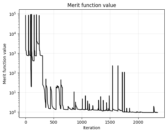
f_val = optimizer.problem.sum_squared()
history.append(f_val)
erf_fig, ax = plt.subplots()
ax.plot(history, color="black")
plt.yscale("log")
ax.set_title("Merit function value")
ax.set_xlabel("Iteration")
ax.set_ylabel("Merit function value")
ax.grid(alpha=0.25)
fig_handle3.update(erf_fig)
plt.close(erf_fig)
# Clear the figure to free memory
del lens_fig # Remove Python reference
del erf_fig # Remove Python reference
import gc
gc.collect() # Force garbage collection
# Optimize the 6 lenses starting point
res = optimizer.run(
num_neighbours=7,
maxiter=100,
tol=1e-6,
callback=callback,
verbose=True,
plot_glass_map=False,
)
# Display the optimized lens
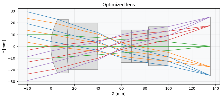
lens.draw(title="Optimized lens")
lens.info()
Show full code listing
python
import optiland.backend as be
from optiland import optic, optimization
from optiland.materials import glasses_selection

target_focal_length = 100  # [mm]


class SixLensesStartPoint(optic.Optic):
  """A 6 lens design with very poor quality meant to be optimized."""

  def __init__(self):
      super().__init__()

      self.add_surface(index=0, radius=be.inf, thickness=be.inf)
      self.add_surface(index=1, radius=1000, thickness=25, material="N-BK7")
      self.add_surface(index=2, radius=1000, thickness=5.0)
      self.add_surface(index=3, radius=1000, thickness=25, material="N-BK7")
      self.add_surface(index=4, radius=be.inf, thickness=25, material="N-BK7")
      self.add_surface(index=5, radius=1000, thickness=25)
      self.add_surface(index=6, radius=be.inf, thickness=25.0, is_stop=True)
      self.add_surface(index=7, radius=-1000, thickness=25, material="N-BK7")
      self.add_surface(index=8, radius=be.inf, thickness=25, material="N-BK7")
      self.add_surface(index=9, radius=-1000, thickness=5.0)
      self.add_surface(index=10, radius=1000, thickness=25, material="N-BK7")
      self.add_surface(index=11, radius=-1000, thickness=200)
      self.add_surface(index=12)

      self.set_aperture(aperture_type="imageFNO", value=5)
      self.set_field_type(field_type="angle")

      self.add_field(y=-14)
      self.add_field(y=-10)
      self.add_field(y=0)
      self.add_field(y=10)
      self.add_field(y=14)

      self.add_wavelength(value=0.4861)
      self.add_wavelength(value=0.5876, is_primary=True)
      self.add_wavelength(value=0.6563)


lens = SixLensesStartPoint()
lens.draw(title="Starting lens")
lens.info()

problem = optimization.OptimizationProblem()

# Real ray height to define the focal length
for k, hy in enumerate([-1, -0.714, 0, 0.714, 1]):
  input_data = {
      "optic": lens,
      "surface_number": 12,
      "Hx": 0,
      "Hy": hy,
      "Px": 0,
      "Py": 0,
      "wavelength": lens.wavelengths.primary_wavelength.value,
  }
  problem.add_operand(
      operand_type="real_y_intercept_lcs",
      target=target_focal_length * be.tan(be.deg2rad(lens.fields.y_fields[k])),
      weight=1,
      input_data=input_data,
  )

# RMS spot size - Minimize the spot size for each field at the primary wavelength.
# We choose a 'uniform' distribution, so the number of rays actually means the rays on
# one axis. Therefore we trace ≈16^2 rays here.
for field in lens.fields.get_field_coords():
  input_data = {
      "optic": lens,
      "surface_number": 12,
      "Hx": field[0],
      "Hy": field[1],
      "num_rays": 16,
      "wavelength": lens.wavelengths.primary_wavelength.value,
      "distribution": "uniform",
  }
  problem.add_operand(
      operand_type="rms_spot_size",
      target=0.0,
      weight=10,
      input_data=input_data,
  )

# Radii
problem.add_variable(lens, "radius", surface_number=1, min_val=-500, max_val=500)
problem.add_variable(lens, "radius", surface_number=2, min_val=-500, max_val=500)
problem.add_variable(lens, "radius", surface_number=3, min_val=-500, max_val=500)
problem.add_variable(lens, "radius", surface_number=5, min_val=-500, max_val=500)
problem.add_variable(lens, "radius", surface_number=7, min_val=-500, max_val=500)
problem.add_variable(lens, "radius", surface_number=9, min_val=-500, max_val=500)
problem.add_variable(lens, "radius", surface_number=10, min_val=-500, max_val=500)
problem.add_variable(lens, "radius", surface_number=11, min_val=-500, max_val=500)

# Thicknesses
problem.add_variable(lens, "thickness", surface_number=1, min_val=8, max_val=20)
problem.add_variable(lens, "thickness", surface_number=2, min_val=0.4, max_val=5)
problem.add_variable(lens, "thickness", surface_number=3, min_val=8, max_val=20)
problem.add_variable(lens, "thickness", surface_number=4, min_val=3, max_val=10)
problem.add_variable(lens, "thickness", surface_number=5, min_val=10, max_val=20)
problem.add_variable(lens, "thickness", surface_number=6, min_val=10, max_val=20)
problem.add_variable(lens, "thickness", surface_number=7, min_val=3, max_val=20)
problem.add_variable(lens, "thickness", surface_number=8, min_val=8, max_val=20)
problem.add_variable(lens, "thickness", surface_number=9, min_val=0.4, max_val=5)
problem.add_variable(lens, "thickness", surface_number=10, min_val=6, max_val=20)
problem.add_variable(lens, "thickness", surface_number=11, min_val=20, max_val=45)

# First option: treat glass indexes as continuous variables
# Fast but produces fictious glasses that later need to be replaced by real glasses
# problem.add_variable(lens, "index", surface_number=1,
#                      wavelength=0.5876, min_val=1.4, max_val=2.0)
# problem.add_variable(lens, "index", surface_number=3,
#                      wavelength=0.5876, min_val=1.4, max_val=2.0)
# problem.add_variable(lens, "index", surface_number=4,
#                      wavelength=0.5876, min_val=1.4, max_val=2.0)
# problem.add_variable(lens, "index", surface_number=7,
#                      wavelength=0.5876, min_val=1.4, max_val=2.0)
# problem.add_variable(lens, "index", surface_number=8,
#                      wavelength=0.5876, min_val=1.4, max_val=2.0)
# problem.add_variable(lens, "index", surface_number=10,
#                      wavelength=0.5876, min_val=1.4, max_val=2.0)

# Second option: use Optiland's Glass Expert to find the best combination
glasses = glasses_selection(0.4, 0.7, catalogs=["schott", "ohara"])
problem.add_variable(lens, "material", surface_number=1, glass_selection=glasses)
problem.add_variable(lens, "material", surface_number=3, glass_selection=glasses)
problem.add_variable(lens, "material", surface_number=4, glass_selection=glasses)
problem.add_variable(lens, "material", surface_number=7, glass_selection=glasses)
problem.add_variable(lens, "material", surface_number=8, glass_selection=glasses)
problem.add_variable(lens, "material", surface_number=10, glass_selection=glasses)

problem.info()

import matplotlib.pyplot as plt
from IPython.display import display

# As the problem has glass variables, we must use GlassExpert
optimizer = optimization.GlassExpert(problem)

# Create persistent outputs
fig_handle1 = display(display_id=True)
fig_handle2 = display(display_id=True)
fig_handle3 = display(display_id=True)

# Draw the starting lens
lens_fig = lens.draw(title="Starting lens")
fig_handle1.update(lens_fig)
plt.close(lens_fig)
print(f"Initial error function value: {problem.initial_value:.1f}")

# Define a callback that is called at each iteration of the local optimizer run.
# Used for vizualization purposes but is not recommended
# as it greatly slows down the optimization.

history = []


def callback(*args):
  # Plot the lens at each merit function call
  lens_fig = lens.draw(title="Lens optimization")
  fig_handle2.update(lens_fig)
  plt.close(lens_fig)

  # Plot merit function evolution
  f_val = optimizer.problem.sum_squared()
  history.append(f_val)
  erf_fig, ax = plt.subplots()
  ax.plot(history, color="black")
  plt.yscale("log")
  ax.set_title("Merit function value")
  ax.set_xlabel("Iteration")
  ax.set_ylabel("Merit function value")
  ax.grid(alpha=0.25)
  fig_handle3.update(erf_fig)
  plt.close(erf_fig)

  # Clear the figure to free memory
  del lens_fig  # Remove Python reference
  del erf_fig  # Remove Python reference
  import gc

  gc.collect()  # Force garbage collection


# Optimize the 6 lenses starting point
res = optimizer.run(
  num_neighbours=7,
  maxiter=100,
  tol=1e-6,
  callback=callback,
  verbose=True,
  plot_glass_map=False,
)

# Display the optimized lens
lens.draw(title="Optimized lens")
lens.info()
Conclusions
- The tutorial demonstrated how to use Optiland's
GlassExpertoptimizer to perform categorical glass selection, automatically choosing the best combination of real glasses from the Schott and Ohara catalogs rather than relying on fictitious continuous-index variables. - A six-element starting design (all N-BK7) was set up deliberately poorly so that the optimizer had meaningful room to improve image quality, illustrating a typical real-world starting-point workflow.
- Material variables were added alongside continuous geometry variables (radii and thicknesses), showing how mixed discrete-continuous optimization problems can be solved within a single
OptimizationProbleminstance. - The
GlassExpert.run()method explored the glass map by testing neighboring glasses at each iteration, providing a convergent path through a fundamentally non-differentiable search space. - A live callback was used to plot the evolving lens layout and merit function history during optimization, demonstrating how to monitor and visualize convergence in an interactive notebook environment.
Next tutorials
NextMulti-Configuration Zoom LensLearn how to handle lenses that change their state and geometry.RelatedMaterial DatabaseReview how to manually browse and load glasses from the internal library.
Original notebook: Tutorial_7e_Glass_Expert.ipynb on GitHub · ReadTheDocs