Case Study

Optimization Case Study

Follow the end-to-end design of a real-world imaging system.

AdvancedOptimizationNumPy backend15 min read

Introduction

This tutorial demonstrates how Optiland can be used to design an F/5 Cooke triplet starting from three (nearly) parallel plates.

Core concepts used

lens.pickups.add(...)

Links one surface parameter to another. Useful for maintaining symmetry or specific air-gap ratios.

optimization.LeastSquares(...)

A fast, gradient-based solver ideal for early-stage design where Seidel targets are the priority.

lens.image_solve()

Automatically adjusts the back-focus distance to place the image plane at the paraxial focus point.

Step-by-step build

Import libraries and define the starting lens

python

import numpy as np

from optiland import analysis, optic, optimization

Define the Cooke Triplet class with surfaces and fields

We start with a system that consists of 3 (nearly) parallel plates, in which all surface have an absolute radius of curvature of 1000 mm. The center element uses glass type F2, while the first and last lens use SK16.

We specify a maximum field of 20 degrees and an entrance pupil diameter of 10 mm. We will later specify a target focal length of 50 mm, which implies an F-number of 5.0 = 50 mm / 10 mm. We'll place the stop on the back side of the center lens.

python

class Triplet(optic.Optic):
 def __init__(self):
     super().__init__()

     # Define surfaces
     self.add_surface(index=0, radius=np.inf, thickness=np.inf)
     self.add_surface(index=1, radius=1000, thickness=4, material="SK16")
     self.add_surface(index=2, radius=-1000, thickness=5)
     self.add_surface(index=3, radius=-1000, thickness=4, material=("F2", "schott"))
     self.add_surface(index=4, radius=1000, thickness=5, is_stop=True)
     self.add_surface(index=5, radius=1000, thickness=4, material="SK16")
     self.add_surface(index=6, radius=-1000, thickness=50)
     self.add_surface(index=7)

     # Define aperture
     self.set_aperture(aperture_type="EPD", value=10.0)

     # Define fields
     self.set_field_type(field_type="angle")
     self.add_field(y=0)
     self.add_field(y=14)
     self.add_field(y=20)

     # Define wavelengths
     self.add_wavelength(value=0.4861)
     self.add_wavelength(value=0.5876, is_primary=True)
     self.add_wavelength(value=0.6563)

Draw the initial lens layout

Let's view the starting point of the lens:

python

lens = Triplet()
fig = lens.draw()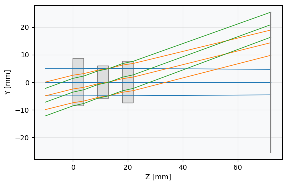

Add symmetry pickups to link surface radii

While technically not required, we will identify a lens starting point that satisfies the required focal length and minimizes the seidel aberrations.

We first specify pickups on the surfaces to enforce symmetry in the design. The first and last lens surfaces should be equal and opposite. Similarly, the second and fifth, as well as third and fourth, should be equal and opposite.

We define this as follows, using a "scale" factor of -1 and an offset of 0. The radius of curvature is defined as $R_\text{new} = R * \text{scale} + \text{offset}$ , where $R$ is the radius of curvature of the reference surface.

python

lens.pickups.add(
 source_surface_idx=1,
 attr_type="radius",
 target_surface_idx=6,
 scale=-1,
 offset=0,
)
lens.pickups.add(
 source_surface_idx=2,
 attr_type="radius",
 target_surface_idx=5,
 scale=-1,
 offset=0,
)
lens.pickups.add(
 source_surface_idx=3,
 attr_type="radius",
 target_surface_idx=4,
 scale=-1,
 offset=0,
)

Set focal length and Seidel aberration operands

Let's define the optimization problem. We first define the focal length and Seidel aberration operands:

python

problem = optimization.OptimizationProblem()

# Add requirement for focal length
problem.add_operand(operand_type="f2", target=50, weight=1, input_data={"optic": lens})

# Add requirements for Seidel aberrations (1 to 5)
for i in range(1, 6):
 problem.add_operand(
     operand_type="seidel",
     target=0,
     weight=10,
     input_data={"optic": lens, "seidel_number": i},
 )

Add radius variables and inspect the problem

Let's define the variables, which are the first 3 surface radii. Recall that the last 3 radii are picked up to these radii, so they do not need to also be specified as variables.

Finally, we view the optimization problem info.

python

problem.add_variable(lens, "radius", surface_number=1, min_val=-1000, max_val=1000)
problem.add_variable(lens, "radius", surface_number=2, min_val=-1000, max_val=1000)
problem.add_variable(lens, "radius", surface_number=3, min_val=-1000, max_val=1000)

problem.info()

Run least-squares optimization for Seidel targets

We then perform optimization. Here, we use the least squares optimizer in Optiland, which simply wraps the implementation in scipy.optimize.least_squares.

python

optimizer = optimization.LeastSquares(problem)
res = optimizer.optimize(
 tol=1e-3, method_choice="trf"
)  # Trust Region Reflective (trf) method supports bounds

Inspect the post-optimization merit function

Let's view the optimization result. We see that there is a >99.99% improvement in the merit function.

python

problem.info()

Apply image solve to set paraxial focus

Before viewing, we call "image_solve" to move the image plane to the paraxial image location.

python

lens.image_solve()

Draw the symmetric optimized lens

python

fig = lens.draw()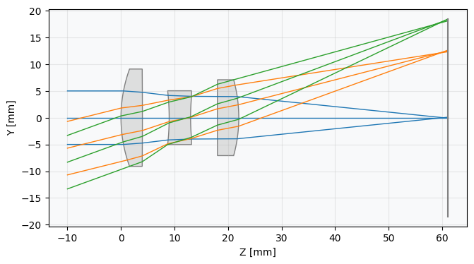

Clear symmetry pickups to free all radii

In the second step, we remove the requirement that the lens is symmetric. We first clear all pickups.

python

lens.pickups.clear()

Switch operands to RMS spot size across all fields

Now that we have a starting design, we will no longer consider the Seidel aberrations. Instead, we will optimize for a minimal RMS spot size for all fields and wavelengths as follows:

python

# Clear all operands
problem.clear_operands()

# focal length requirement
problem.add_operand(operand_type="f2", target=50, weight=1, input_data={"optic": lens})

# RMS spot size requirement at (0, 0) field
input_data = {
 "optic": lens,
 "surface_number": -1,
 "Hx": 0,
 "Hy": 0,
 "wavelength": "all",
 "num_rays": 5,
}
problem.add_operand(
 operand_type="rms_spot_size",
 target=0,
 weight=10,
 input_data=input_data,
)

# RMS spot size requirement at (0, 0.7) field
input_data = {
 "optic": lens,
 "surface_number": -1,
 "Hx": 0,
 "Hy": 0.7,
 "wavelength": "all",
 "num_rays": 5,
}
problem.add_operand(
 operand_type="rms_spot_size",
 target=0,
 weight=10,
 input_data=input_data,
)

# RMS spot size requirement at (0, 1.0) field
input_data = {
 "optic": lens,
 "surface_number": -1,
 "Hx": 0,
 "Hy": 1.0,
 "wavelength": "all",
 "num_rays": 5,
}
problem.add_operand(
 operand_type="rms_spot_size",
 target=0,
 weight=10,
 input_data=input_data,
)

Expand variables to include remaining radii and back focus

We add the last 3 radii as variables, as well as the thickness to the image plane.

python

problem.add_variable(lens, "radius", surface_number=4, min_val=-1000, max_val=1000)
problem.add_variable(lens, "radius", surface_number=5, min_val=-1000, max_val=1000)
problem.add_variable(lens, "radius", surface_number=6, min_val=-1000, max_val=1000)

problem.add_variable(lens, "thickness", surface_number=6, min_val=0, max_val=1000)

problem.info()

Run generic optimizer on RMS spot size

Let's optimize the system, view the result and plot the lens. In this iteration, we use the generic optimizer in Optiland, which wraps scipy.optimize.minimmize.

python

optimizer = optimization.OptimizerGeneric(problem)
res = optimizer.optimize(tol=1e-9)

Inspect merit function after RMS optimization

python

problem.info()

Draw the lens after RMS spot optimization

python

fig = lens.draw()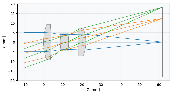

Add air-gap thicknesses as fine-tuning variables

As a last step, we will let the thicknesses between the lenses vary and re-optimize. Allowing the lens thicknesses to vary is generally unnecessary, as it offers very little corrective power.

python

problem.add_variable(lens, "thickness", surface_number=2, min_val=1, max_val=10)
problem.add_variable(lens, "thickness", surface_number=4, min_val=1, max_val=10)

Inspect the expanded variable set

python

problem.info()

Run final optimization with all variables

Let's optimize the system one last time with all variables to fine tune the system.

python

optimizer = optimization.OptimizerGeneric(problem)
res = optimizer.optimize(tol=1e-9)

Inspect the final merit function

python

problem.info()

Draw the final optimized Cooke Triplet

python

fig = lens.draw()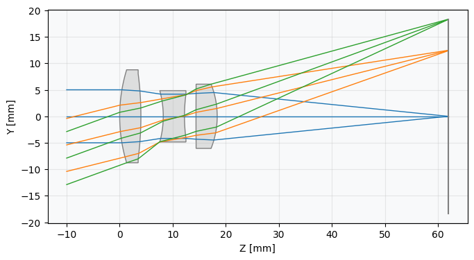

View the spot diagram for all fields

We view the spot diagram to see the final performance of our system.

python

spot = analysis.SpotDiagram(lens)
spot.view()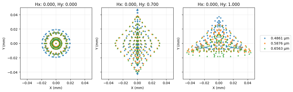

Print RMS spot radii per field and wavelength

And we print the RMS spot radii for each wavelength and field.

python

print("RMS Spot Radius:")

fields = lens.fields.get_field_coords()
wavelengths = lens.wavelengths.get_wavelengths()

rms_spot_radius = spot.rms_spot_radius()
for i, field in enumerate(fields):
 for j, wavelength in enumerate(wavelengths):
     print(
         f"\tField {field}, Wavelength {wavelength:.3f} µm, "
         f"Radius: {rms_spot_radius[i][j]:.5f} mm",
     )

Show full code listing

python

import numpy as np

from optiland import analysis, optic, optimization

class Triplet(optic.Optic):
  def __init__(self):
      super().__init__()

      # Define surfaces
      self.add_surface(index=0, radius=np.inf, thickness=np.inf)
      self.add_surface(index=1, radius=1000, thickness=4, material="SK16")
      self.add_surface(index=2, radius=-1000, thickness=5)
      self.add_surface(index=3, radius=-1000, thickness=4, material=("F2", "schott"))
      self.add_surface(index=4, radius=1000, thickness=5, is_stop=True)
      self.add_surface(index=5, radius=1000, thickness=4, material="SK16")
      self.add_surface(index=6, radius=-1000, thickness=50)
      self.add_surface(index=7)

      # Define aperture
      self.set_aperture(aperture_type="EPD", value=10.0)

      # Define fields
      self.set_field_type(field_type="angle")
      self.add_field(y=0)
      self.add_field(y=14)
      self.add_field(y=20)

      # Define wavelengths
      self.add_wavelength(value=0.4861)
      self.add_wavelength(value=0.5876, is_primary=True)
      self.add_wavelength(value=0.6563)

lens = Triplet()
fig = lens.draw()

lens.pickups.add(
  source_surface_idx=1,
  attr_type="radius",
  target_surface_idx=6,
  scale=-1,
  offset=0,
)
lens.pickups.add(
  source_surface_idx=2,
  attr_type="radius",
  target_surface_idx=5,
  scale=-1,
  offset=0,
)
lens.pickups.add(
  source_surface_idx=3,
  attr_type="radius",
  target_surface_idx=4,
  scale=-1,
  offset=0,
)

problem = optimization.OptimizationProblem()

# Add requirement for focal length
problem.add_operand(operand_type="f2", target=50, weight=1, input_data={"optic": lens})

# Add requirements for Seidel aberrations (1 to 5)
for i in range(1, 6):
  problem.add_operand(
      operand_type="seidel",
      target=0,
      weight=10,
      input_data={"optic": lens, "seidel_number": i},
  )

problem.add_variable(lens, "radius", surface_number=1, min_val=-1000, max_val=1000)
problem.add_variable(lens, "radius", surface_number=2, min_val=-1000, max_val=1000)
problem.add_variable(lens, "radius", surface_number=3, min_val=-1000, max_val=1000)

problem.info()

optimizer = optimization.LeastSquares(problem)
res = optimizer.optimize(
  tol=1e-3, method_choice="trf"
)  # Trust Region Reflective (trf) method supports bounds

problem.info()

lens.image_solve()

fig = lens.draw()

lens.pickups.clear()

# Clear all operands
problem.clear_operands()

# focal length requirement
problem.add_operand(operand_type="f2", target=50, weight=1, input_data={"optic": lens})

# RMS spot size requirement at (0, 0) field
input_data = {
  "optic": lens,
  "surface_number": -1,
  "Hx": 0,
  "Hy": 0,
  "wavelength": "all",
  "num_rays": 5,
}
problem.add_operand(
  operand_type="rms_spot_size",
  target=0,
  weight=10,
  input_data=input_data,
)

# RMS spot size requirement at (0, 0.7) field
input_data = {
  "optic": lens,
  "surface_number": -1,
  "Hx": 0,
  "Hy": 0.7,
  "wavelength": "all",
  "num_rays": 5,
}
problem.add_operand(
  operand_type="rms_spot_size",
  target=0,
  weight=10,
  input_data=input_data,
)

# RMS spot size requirement at (0, 1.0) field
input_data = {
  "optic": lens,
  "surface_number": -1,
  "Hx": 0,
  "Hy": 1.0,
  "wavelength": "all",
  "num_rays": 5,
}
problem.add_operand(
  operand_type="rms_spot_size",
  target=0,
  weight=10,
  input_data=input_data,
)

problem.add_variable(lens, "radius", surface_number=4, min_val=-1000, max_val=1000)
problem.add_variable(lens, "radius", surface_number=5, min_val=-1000, max_val=1000)
problem.add_variable(lens, "radius", surface_number=6, min_val=-1000, max_val=1000)

problem.add_variable(lens, "thickness", surface_number=6, min_val=0, max_val=1000)

problem.info()

optimizer = optimization.OptimizerGeneric(problem)
res = optimizer.optimize(tol=1e-9)

problem.info()

fig = lens.draw()

problem.add_variable(lens, "thickness", surface_number=2, min_val=1, max_val=10)
problem.add_variable(lens, "thickness", surface_number=4, min_val=1, max_val=10)

problem.info()

optimizer = optimization.OptimizerGeneric(problem)
res = optimizer.optimize(tol=1e-9)

problem.info()

fig = lens.draw()

spot = analysis.SpotDiagram(lens)
spot.view()

print("RMS Spot Radius:")

fields = lens.fields.get_field_coords()
wavelengths = lens.wavelengths.get_wavelengths()

rms_spot_radius = spot.rms_spot_radius()
for i, field in enumerate(fields):
  for j, wavelength in enumerate(wavelengths):
      print(
          f"\tField {field}, Wavelength {wavelength:.3f} µm, "
          f"Radius: {rms_spot_radius[i][j]:.5f} mm",
      )

Conclusions

Starting from a simple system consisting of 3 (nearly) parallel plates, we designed a Cooke triplet. The triplet achieves an RMS spot size of ≈20 µm or less for all wavelengths and fields. We could have optimized the system to improve the performance further.
We optimized for minimal RMS spot size, but we could have instead chosen to optimize the wavefront or other performance metrics. All operand possibilities can be seen in the operands module.
This tutorial showed a typical example of optimizing an optical system from a simple starting point to a system with significantly improved performance. Lens optimization is complex and can be considered somewhat of an "art". With experience, the lens designer will learn how best to optimize lens systems to achieve target performance.

Next tutorials

NextCustom Optimization OperandsWrite your own Python functions to guide the optimizer.RelatedAdvanced OptimizationReview the global optimization algorithms used for complex designs.

Original notebook: Tutorial_5c_Optimization_Case_Study.ipynb on GitHub · ReadTheDocs