Introduction to Polarization
Track the vector state of light as it interacts with birefringent elements.
Introduction
This tutorial introduces the concept of polarization in Optiland. In particular, we will first assess how the input polarization state impacts the transmission of the nominal system. Then, we will analyze the transmission of an optical system with polarizing coatings applied.
Core concepts used
Step-by-step build
Import Libraries
import matplotlib.pyplot as plt
import numpy as np

from optiland.rays import PolarizationState, create_polarization
from optiland.samples.objectives import ObjectiveUS008879901Load and Draw the Objective Lens
We will use an objective consisting of 12 lens elements for this tutorial:
lens = ObjectiveUS008879901()
lens.draw()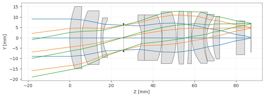
Define Pupil Transmission Helper
Remarks on polarization in Optiland:
-
By default, polarization is entirely ignored
-
There are 3 options for polarization in Optiland:
- Ignore polarization entirely
- Consider a specific polarization state
- Use unpolarized light
These are listed approximately in their order of computation speed, as each subsequent type requires more calculations. Using unpolarized light requires two orthogonal polarization states to be considered and the average transmission of both states is used to update ray transmission.
More information can be found in the Optiland documentation. Let's now start analyzing our system.
To begin, we will create a helper function that plots transmission through our lens (object to image) at the aperture stop level. Plotting the transmission in this way enables us to see pupil-dependent transmission variations.
def plot_transmission(lens, vmin=None, vmax=None):
 fig, axs = plt.subplots(1, 2, figsize=(12, 5))

 # Plot for Hy=0
 rays = lens.trace(
     Hx=0,
     Hy=0,
     wavelength=0.5875618,
     num_rays=256,
     distribution="uniform",
 )
 stop_idx = lens.surface_group.stop_index
 x_stop = lens.surface_group.x[stop_idx, :]
 y_stop = lens.surface_group.y[stop_idx, :]
 r_max = np.max(np.sqrt(x_stop**2 + y_stop**2))
 x_stop /= r_max
 y_stop /= r_max
 axs[0].scatter(x_stop, y_stop, c=rays.i, s=5, vmin=vmin, vmax=vmax)
 axs[0].axis("equal")
 axs[0].set_xlabel("Pupil X")
 axs[0].set_ylabel("Pupil Y")
 axs[0].set_title("Pupil-level Transmission: (Hx, Hy) = (0, 0)")

 cbar = fig.colorbar(axs[0].collections[0])
 cbar.set_label("Transmission", rotation=270, labelpad=20)

 # Plot for Hy=1
 rays = lens.trace(
     Hx=0,
     Hy=1,
     wavelength=0.5875618,
     num_rays=256,
     distribution="uniform",
 )
 stop_idx = lens.surface_group.stop_index
 x_stop = lens.surface_group.x[stop_idx, :]
 y_stop = lens.surface_group.y[stop_idx, :]
 r_max = np.max(np.sqrt(x_stop**2 + y_stop**2))
 x_stop /= r_max
 y_stop /= r_max
 axs[1].scatter(x_stop, y_stop, c=rays.i, s=5, vmin=vmin, vmax=vmax)
 axs[1].axis("equal")
 axs[1].set_xlabel("Pupil X")
 axs[1].set_ylabel("Pupil Y")
 axs[1].set_title("Pupil-level Transmission: (Hx, Hy) = (0, 1)")

 cbar = fig.colorbar(axs[1].collections[0])
 cbar.set_label("Transmission", rotation=270, labelpad=20)

 plt.tight_layout()
plt.show()Apply Fresnel Coatings to All Surfaces
Next, we assign Fresnel coatings to all surfaces, simulating uncoated lenses. We can do this easily using the set_fresnel_coatings method:
lens.surface_group.set_fresnel_coatings()Inspect Default Polarization State
Before we can assess the polarization impact, we must also set our polarization state. As mentioned, the lens defaults to ignoring polarization, which we can see by printing the lens "polarization" attribute:
lens.polarizationSet Unpolarized Light Mode
Let's specify that the lens should use unpolarized light. This can be done using the PolarizationState class:
state = PolarizationState(is_polarized=False)
lens.updater.set_polarization(state)Confirm Updated Polarization State
And we now see that the polarization attribute has changed:
lens.polarizationPlot Fresnel Transmission Map
Let's plot the transmission versus pupil position:
plot_transmission(lens)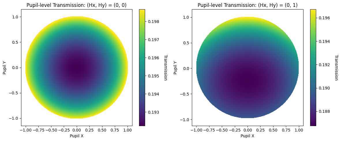
Define a Custom Jones Vector State
The transmission has now dropped considerably. Ignoring polarization, the transmission was 98% and it is now 19%. We see a variation in transmission with both pupil position and field coordinate. Note that the variation in transmission is significantly larger here than in the nominal case.
Instead of using unpolarized light, we can also apply a specific polarization state. This is defined using the Jones vector approach, in which the electric field amplitude and phase are defined in the X and Y axes. Namely, we define
where and are the field amplitudes in x and y, respectively, and and are the phases.
This 2D formulation of the electric field is first converted into 3D based on the ray direction. The exact details of this conversion are out of the scope of this tutorial, but more information can be found in the code documentation.
We define these four components as follows. Note that for simplicity, we drop the "0" subscript of the amplitude.
Ex = 1
Ey = 0.5
phase_x = 0.2
phase_y = 0

state = PolarizationState(
 is_polarized=True,
 Ex=Ex,
 Ey=Ey,
 phase_x=phase_x,
 phase_y=phase_y,
)Trace Rays for Custom Polarization
Testing polarization effects in Optiland
- Due to how Optiland considers polarization, it is only necessary to trace rays a single time before testing the system under different polarization states
We will demonstrate this behavior here. First, we trace a uniform grid of rays at normalized field point (0, 1). The trace function returns the traced rays:
rays = lens.trace(
 Hx=0,
 Hy=1,
 wavelength=0.5875618,
 num_rays=256,
 distribution="uniform",
)Update Ray Intensities with Custom State
Now we can assign our previously-defined polarization state to the rays:
rays.update_intensity(state)Plot Custom Polarization Transmission
And as was done previously, we view the stop-level transmission for our specific polarization state:
stop_idx = lens.surface_group.stop_index
x_stop = lens.surface_group.x[stop_idx, :]
y_stop = lens.surface_group.y[stop_idx, :]
r_max = np.max(np.sqrt(x_stop**2 + y_stop**2))
x_stop /= r_max
y_stop /= r_max

plt.scatter(x_stop, y_stop, c=rays.i, s=5)
plt.axis("equal")
plt.xlabel("Pupil X")
plt.ylabel("Pupil Y")
plt.title("Custom Polarization State")
cbar = plt.colorbar()
cbar.set_label("Transmission", rotation=270, labelpad=20)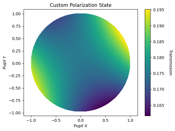
Compare Multiple Polarization States
Lastly, let's demonstrate how to quickly assess different polarization states without the need to re-trace rays.
Here, we make use of the "create_polarization" function, which generates the PolarizationState instance for common polarization types.
fig, axs = plt.subplots(2, 2, figsize=(10, 7))

stop_idx = lens.surface_group.stop_index
x_stop = lens.surface_group.x[stop_idx, :]
y_stop = lens.surface_group.y[stop_idx, :]
r_max = np.max(np.sqrt(x_stop**2 + y_stop**2))
x_stop /= r_max
y_stop /= r_max

for i, pol_type in enumerate(["H", "V", "L+45", "RCP"]):
 state = create_polarization(pol_type)
 lens.updater.set_polarization(state)
 rays.update_intensity(state)

 ax = axs[i // 2, i % 2]
 scatter = ax.scatter(x_stop, y_stop, c=rays.i, s=5)
 ax.axis("equal")
 ax.set_title(f"Polarization: {pol_type}")
 ax.set_xlabel("Pupil X")
 ax.set_ylabel("Pupil Y")

 cbar = fig.colorbar(scatter, ax=ax)
 cbar.set_label("Transmission", rotation=270, labelpad=20)

plt.tight_layout()
plt.show()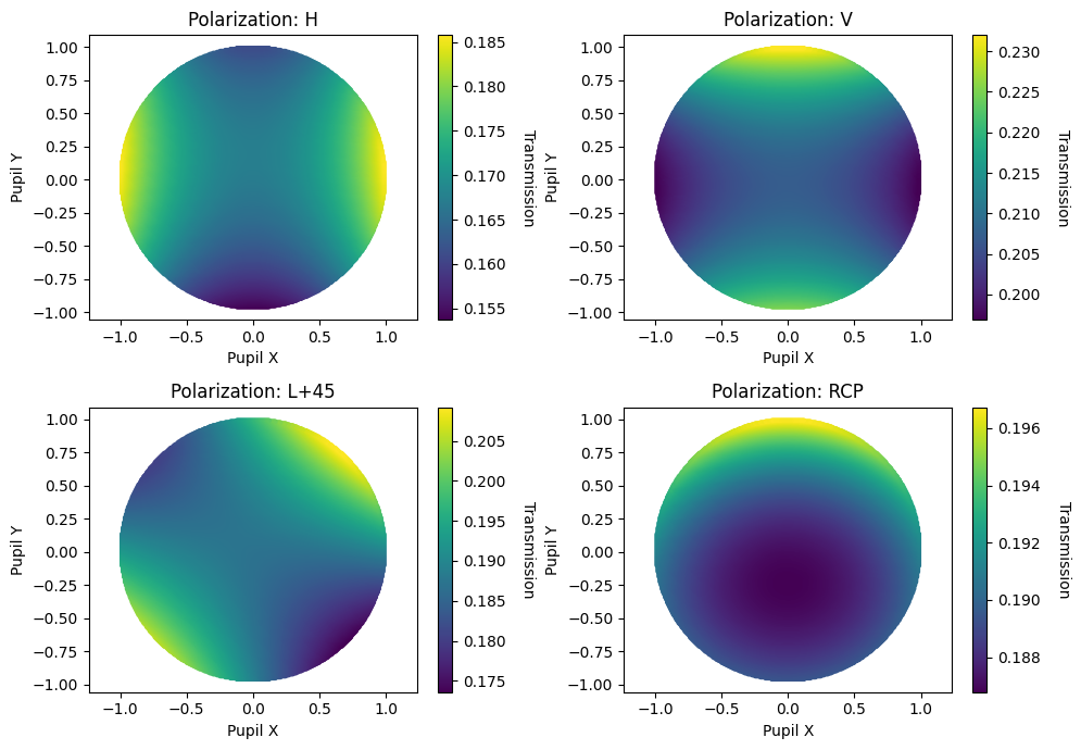
Modeling Polarizers and Retarders
We can also add specific polarizing coatings to our surfaces. For instance, we may wish to model a linear polarizer applied to one of our optical components.
from optiland.coatings import PolarizerCoating

# Let's place a vertical polarizer on the 4th surface (along y-axis)
pol_v = PolarizerCoating(axis=(0.0, 1.0, 0.0))
# <-- manually add coating here (not recommended - see below)
lens.surface_group.surfaces[4].interaction_model.coating = pol_vDefine Coating During Surface Creation
Note that in the typical setup, you would define the coating during the creation of a surface, as shown here:
lens = Optic()


# ...
lens.add_surface(
 index=4,  # let's say we're adding the coating to the 4th surface
 thickness=10.0,
 is_stop=True,
 material="F2",
 coating=PolarizerCoating(axis=(0.0, 1.0, 0.0)),  # <-- add coating here
)
# ... define rest of the optic
Both PolarizerCoating and RetarderCoating can be used to define polarization-sensitive coatings. The former is used for polarizers, while the latter is used for retarders. See API documentation for more details.
Now, let's re-trace the unpolarized light and see the transmission profile, which is now affected by the linear polarizer:
state = PolarizationState(is_polarized=False)
lens.updater.set_polarization(state)
plot_transmission(lens)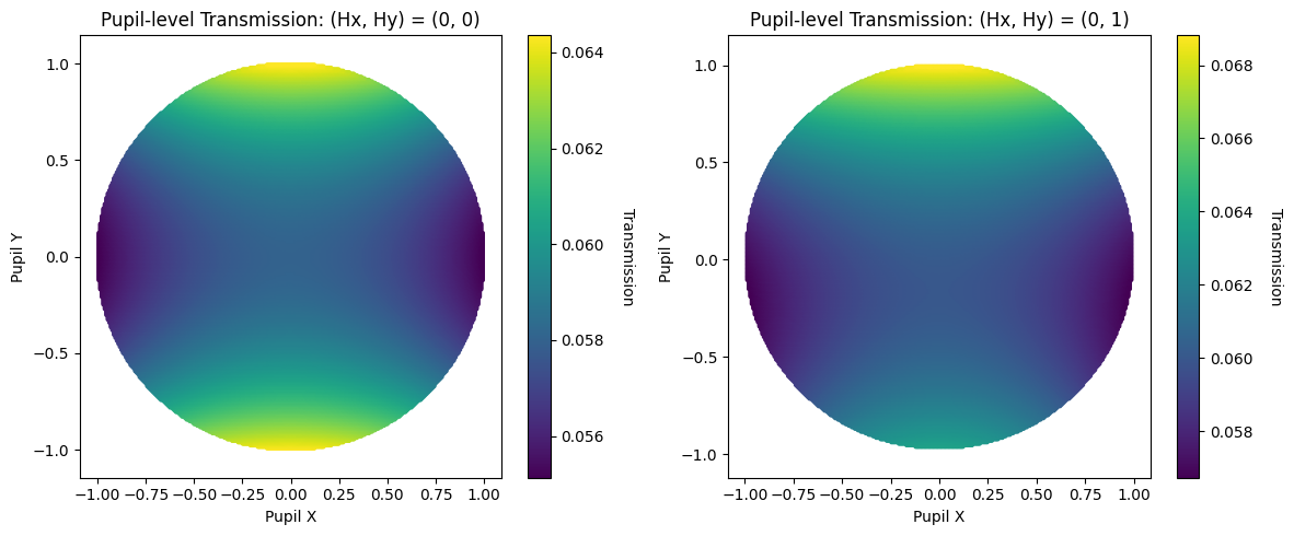
Show full code listing
import matplotlib.pyplot as plt
import numpy as np

from optiland.rays import PolarizationState, create_polarization
from optiland.samples.objectives import ObjectiveUS008879901

lens = ObjectiveUS008879901()
lens.draw()

def plot_transmission(lens, vmin=None, vmax=None):
  fig, axs = plt.subplots(1, 2, figsize=(12, 5))

  # Plot for Hy=0
  rays = lens.trace(
      Hx=0,
      Hy=0,
      wavelength=0.5875618,
      num_rays=256,
      distribution="uniform",
  )
  stop_idx = lens.surface_group.stop_index
  x_stop = lens.surface_group.x[stop_idx, :]
  y_stop = lens.surface_group.y[stop_idx, :]
  r_max = np.max(np.sqrt(x_stop**2 + y_stop**2))
  x_stop /= r_max
  y_stop /= r_max
  axs[0].scatter(x_stop, y_stop, c=rays.i, s=5, vmin=vmin, vmax=vmax)
  axs[0].axis("equal")
  axs[0].set_xlabel("Pupil X")
  axs[0].set_ylabel("Pupil Y")
  axs[0].set_title("Pupil-level Transmission: (Hx, Hy) = (0, 0)")

  cbar = fig.colorbar(axs[0].collections[0])
  cbar.set_label("Transmission", rotation=270, labelpad=20)

  # Plot for Hy=1
  rays = lens.trace(
      Hx=0,
      Hy=1,
      wavelength=0.5875618,
      num_rays=256,
      distribution="uniform",
  )
  stop_idx = lens.surface_group.stop_index
  x_stop = lens.surface_group.x[stop_idx, :]
  y_stop = lens.surface_group.y[stop_idx, :]
  r_max = np.max(np.sqrt(x_stop**2 + y_stop**2))
  x_stop /= r_max
  y_stop /= r_max
  axs[1].scatter(x_stop, y_stop, c=rays.i, s=5, vmin=vmin, vmax=vmax)
  axs[1].axis("equal")
  axs[1].set_xlabel("Pupil X")
  axs[1].set_ylabel("Pupil Y")
  axs[1].set_title("Pupil-level Transmission: (Hx, Hy) = (0, 1)")

  cbar = fig.colorbar(axs[1].collections[0])
  cbar.set_label("Transmission", rotation=270, labelpad=20)

  plt.tight_layout()
  plt.show()

lens.surface_group.set_fresnel_coatings()

lens.polarization

state = PolarizationState(is_polarized=False)
lens.updater.set_polarization(state)

lens.polarization

plot_transmission(lens)

Ex = 1
Ey = 0.5
phase_x = 0.2
phase_y = 0

state = PolarizationState(
  is_polarized=True,
  Ex=Ex,
  Ey=Ey,
  phase_x=phase_x,
  phase_y=phase_y,
)

rays = lens.trace(
  Hx=0,
  Hy=1,
  wavelength=0.5875618,
  num_rays=256,
  distribution="uniform",
)

rays.update_intensity(state)

stop_idx = lens.surface_group.stop_index
x_stop = lens.surface_group.x[stop_idx, :]
y_stop = lens.surface_group.y[stop_idx, :]
r_max = np.max(np.sqrt(x_stop**2 + y_stop**2))
x_stop /= r_max
y_stop /= r_max

plt.scatter(x_stop, y_stop, c=rays.i, s=5)
plt.axis("equal")
plt.xlabel("Pupil X")
plt.ylabel("Pupil Y")
plt.title("Custom Polarization State")
cbar = plt.colorbar()
cbar.set_label("Transmission", rotation=270, labelpad=20)

fig, axs = plt.subplots(2, 2, figsize=(10, 7))

stop_idx = lens.surface_group.stop_index
x_stop = lens.surface_group.x[stop_idx, :]
y_stop = lens.surface_group.y[stop_idx, :]
r_max = np.max(np.sqrt(x_stop**2 + y_stop**2))
x_stop /= r_max
y_stop /= r_max

for i, pol_type in enumerate(["H", "V", "L+45", "RCP"]):
  state = create_polarization(pol_type)
  lens.updater.set_polarization(state)
  rays.update_intensity(state)

  ax = axs[i // 2, i % 2]
  scatter = ax.scatter(x_stop, y_stop, c=rays.i, s=5)
  ax.axis("equal")
  ax.set_title(f"Polarization: {pol_type}")
  ax.set_xlabel("Pupil X")
  ax.set_ylabel("Pupil Y")

  cbar = fig.colorbar(scatter, ax=ax)
  cbar.set_label("Transmission", rotation=270, labelpad=20)

plt.tight_layout()
plt.show()

from optiland.coatings import PolarizerCoating

# Let's place a vertical polarizer on the 4th surface (along y-axis)
pol_v = PolarizerCoating(axis=(0.0, 1.0, 0.0))
# <-- manually add coating here (not recommended - see below)
lens.surface_group.surfaces[4].interaction_model.coating = pol_v

state = PolarizationState(is_polarized=False)
lens.updater.set_polarization(state)
plot_transmission(lens)
Conclusions
Conclusions
- This tutorial demonstrated polarization functionality in Optiland.
- Optiland requires that rays only be traced once before various polarization types are assessed.
In future tutorials, we will expand on polarization topics, including the Jones pupil and advanced coating designs.
Next tutorials
Original notebook: Tutorial_6b_Introduction_to_Polarization.ipynb on GitHub · ReadTheDocs