Custom Optimization Algorithms
Implement your own search strategy, from random walks to custom heuristics.
Introduction
This tutorial demonstrates how to define a custom optimization algorithm in Optiland. There are already several optimization algorithms available in Optiland, including a least squares optimizer, dual annealing, differential evolution, and a generic optimizer that wraps scipy.optimize.minimize. While the existing algorithms may cover most use cases, it is sometimes necessary to implement a custom algorithm to meet specific requirements.
In this tutorial, we will create a random walk optimizer, which traverses the design space by making random steps and evaluating the objective function at each step. This is a very simple (and inefficient) strategy for optimization, but it will demonstrate how to integrate a custom algorithm into the Optiland framework.
Core concepts used
Step-by-step build
Import Required Modules
import matplotlib.pyplot as plt
import numpy as np

from optiland import analysis, optic, optimizationDefine the Aspheric Singlet Lens
Our goal will be to optimize the coefficients of an aspheric singlet to minimize the RMS spot size. We start by first defining this singlet with all aspheric coefficients set to zero.
class AsphericSinglet(optic.Optic):
 """Aspheric singlet"""

 def __init__(self):
     super().__init__()

     # add surfaces
     self.add_surface(index=0, radius=np.inf, thickness=np.inf)
     self.add_surface(
         index=1,
         thickness=7,
         radius=20.0,
         is_stop=True,
         material="N-SF11",
         surface_type="even_asphere",
         conic=0.0,
         coefficients=[0, 0, 0],
     )
     self.add_surface(index=2, thickness=21.56201105)
     self.add_surface(index=3)

     # add aperture
     self.set_aperture(aperture_type="EPD", value=20.0)

     # add field
     self.set_field_type(field_type="angle")
     self.add_field(y=0)

     # add wavelength
self.add_wavelength(value=0.55, is_primary=True)Implement the Random Walk Optimizer
Next, we need to define our optimization algorithm. This is a class that inherits from optimization.OptimizerGeneric. This class has two requirements:
- The constructor must accept the optimization problem as an argument. This is an instance of
optimization.OptimizationProblem. - The class must implement the
optimizemethod.
The optimization algorithm is as follows:
-
Get current variable values ("position") and the objective function value.
-
Save the initial position in case we want to undo the optimization later (optional, but good practice).
-
Generate a random step.
-
Calculate the objective function at the new position.
-
If the new position is better, accept the step.
-
Continue for the maximum number of steps.
-
Update the variables to the optimal position.
pythonclass RandomWalkOptimizer(optimization.OptimizerGeneric): def __init__(self, problem): super().__init__(problem) def optimize(self, max_steps=100, delta=0.1, seed=42): # Set random seed np.random.seed(seed) # Get current position and objective function value current_position = [var.value for var in self.problem.variables] current_value = self._fun(current_position) num_variables = len(current_position) # save initial position to be able to revert self._x.append(current_position) # Save values of each iteration values = [current_value] for _ in range(max_steps): # Generate a random step random_step = np.random.randn(num_variables) * delta new_position = current_position + random_step # Calculate the objective function value at the new position new_value = self._fun(new_position) values.append(new_value) # If the new value is better, accept the step if new_value < current_value: current_position = new_position current_value = new_value # Update the variables with the best position for idvar, var in enumerate(self.problem.variables): var.update(current_position[idvar]) return values
Draw the Starting Lens
Let's create and draw the starting point lens.
lens = AsphericSinglet()
lens.draw(num_rays=5)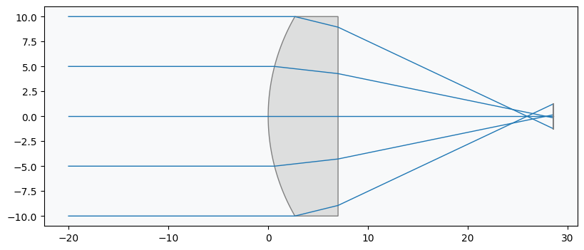
Create the Optimization Problem
We now create the optimization problem, add our operand (RMS spot size target) and variables (3 aspheric coefficients).
problem = optimization.OptimizationProblem()Add the RMS Spot Size Operand
input_data = {
"optic": lens,
"surface_number": -1,
"Hx": 0,
"Hy": 0,
"num_rays": 5,
"wavelength": 0.55,
"distribution": "hexapolar",
}
# add RMS spot size operand
problem.add_operand(
operand_type="rms_spot_size",
target=0,
weight=1,
input_data=input_data,
)Add Aspheric Coefficient Variables
problem.add_variable(lens, "asphere_coeff", surface_number=1, coeff_number=0)
problem.add_variable(lens, "asphere_coeff", surface_number=1, coeff_number=1)
problem.add_variable(lens, "asphere_coeff", surface_number=1, coeff_number=2)Inspect the Problem Configuration
We print the optimization problem info to see the current status.
problem.info()Instantiate the Optimizer
Let's now create an optimizer using our RandomWalkOptimizer class. We pass the optimization problem as an argument.
optimizer = RandomWalkOptimizer(problem)Run the Optimization
Finally, we can run the optimization by calling the optimize. We choose to run the optimization for 1000 steps and use a delta value of 0.1. The delta value controls the size of the step in each iteration.
values = optimizer.optimize(max_steps=1000, delta=0.1)Review Results
On the author's machine, the optimization completes in 2 seconds. Let's print the problem information to see whether optimization was successful.
problem.info()Draw the Optimized Lens
Indeed, the objective function value is minimized. We also draw the lens and generate the spot diagram to confirm.
lens.draw(num_rays=5)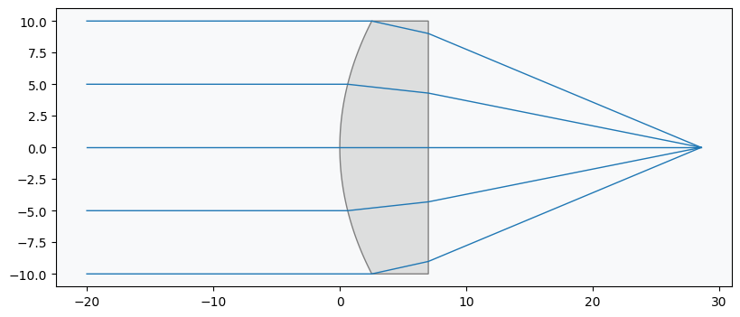
Generate the Optimized Spot Diagram
spot = analysis.SpotDiagram(lens)
spot.view()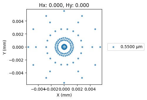
Plot Optimizer Convergence
Recall that we also saved the values of the objective function in each iteration. We can now use these values to plot the convergence of the objective function over the 1000 iterations.
plt.plot(values)
plt.xlabel("Iteration")
plt.ylabel("Objective Function Value")
plt.title("Convergence of Random Walk Optimizer")
plt.grid(True)
plt.show()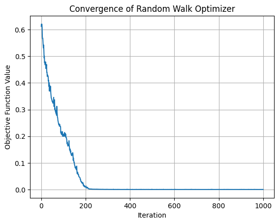
We can clearly see that the optimization converges within about 250 iterations. We can therefore conclude that the random walk optimizer is effective for this problem. For improved performance, we might consider adding a stopping condition in the future to avoid unnecessary iterations.
Show full code listing
import matplotlib.pyplot as plt
import numpy as np
from optiland import analysis, optic, optimization
class AsphericSinglet(optic.Optic):
"""Aspheric singlet"""
def __init__(self):
super().__init__()
# add surfaces
self.add_surface(index=0, radius=np.inf, thickness=np.inf)
self.add_surface(
index=1,
thickness=7,
radius=20.0,
is_stop=True,
material="N-SF11",
surface_type="even_asphere",
conic=0.0,
coefficients=[0, 0, 0],
)
self.add_surface(index=2, thickness=21.56201105)
self.add_surface(index=3)
# add aperture
self.set_aperture(aperture_type="EPD", value=20.0)
# add field
self.set_field_type(field_type="angle")
self.add_field(y=0)
# add wavelength
self.add_wavelength(value=0.55, is_primary=True)
class RandomWalkOptimizer(optimization.OptimizerGeneric):
 def __init__(self, problem):
     super().__init__(problem)

 def optimize(self, max_steps=100, delta=0.1, seed=42):
     # Set random seed
     np.random.seed(seed)

     # Get current position and objective function value
     current_position = [var.value for var in self.problem.variables]
     current_value = self._fun(current_position)
     num_variables = len(current_position)

     # save initial position to be able to revert
     self._x.append(current_position)

     # Save values of each iteration
     values = [current_value]

     for _ in range(max_steps):
         # Generate a random step
         random_step = np.random.randn(num_variables) * delta
         new_position = current_position + random_step

         # Calculate the objective function value at the new position
         new_value = self._fun(new_position)
         values.append(new_value)

         # If the new value is better, accept the step
         if new_value < current_value:
             current_position = new_position
             current_value = new_value

     # Update the variables with the best position
     for idvar, var in enumerate(self.problem.variables):
         var.update(current_position[idvar])

     return values
lens = AsphericSinglet()
lens.draw(num_rays=5)
problem = optimization.OptimizationProblem()
input_data = {
 "optic": lens,
 "surface_number": -1,
 "Hx": 0,
 "Hy": 0,
 "num_rays": 5,
 "wavelength": 0.55,
 "distribution": "hexapolar",
}

# add RMS spot size operand
problem.add_operand(
 operand_type="rms_spot_size",
 target=0,
 weight=1,
 input_data=input_data,
)
problem.add_variable(lens, "asphere_coeff", surface_number=1, coeff_number=0)
problem.add_variable(lens, "asphere_coeff", surface_number=1, coeff_number=1)
problem.add_variable(lens, "asphere_coeff", surface_number=1, coeff_number=2)
problem.info()
optimizer = RandomWalkOptimizer(problem)
values = optimizer.optimize(max_steps=1000, delta=0.1)
problem.info()
lens.draw(num_rays=5)
spot = analysis.SpotDiagram(lens)
spot.view()
plt.plot(values)
plt.xlabel("Iteration")
plt.ylabel("Objective Function Value")
plt.title("Convergence of Random Walk Optimizer")
plt.grid(True)
plt.show()Conclusions
- This tutorial showed how to add custom optimization algorithms in Optiland.
- A custom optimizer inherits from
optimization.OptimizerGenericand it must 1) accept the optimization problem as an argument and 2) implement theoptimizemethod. - The methods shown here can be used to define any arbitrary optimization algorithm. Likewise, existing optimization libraries can be built into Optiland using this approach.
Next tutorials
Original notebook: Tutorial_10c_Custom_Optimization_Algorithm.ipynb on GitHub · ReadTheDocs