Thin Films

Color Analysis for Thin-Films

Perceive the visual appearance of coatings using colorimetry tools.

IntermediateCoatings & PolarizationNumPy backend12 min read

Introduction

This example shows how the reflected color of a TiO2 thin film on silica evolves with thickness. We compute chromaticity coordinates from a normalized reflected spectrum and visualize the path on the CIE 1931 diagram, then summarize the color evolution with a thickness color bar.

Goals

Compute $x, y$ chromaticity for a TiO2 layer on SiO2.
Trace the chromaticity path for thicknesses from 0 to 250 nm.
Visualize the perceived color as a function of thickness.

Core concepts used

stack.reflectance_nm_deg(...)

Calculates the full spectral reflectance, the "fingerprint" of the coating's color.

SpectralAnalyzer

The core analysis class for computing perception-based color coordinates (XYZ, xyY, sRGB) from thin-film spectra.

plot_cie_1931_chromaticity_diagram()

A specialized plotter for visualizing the standard human color gamut background.

thickness_sweep

Iterating through design parameters to visualize continuous behavior changes.

Step-by-step build

Import colorimetry and thin-film libraries

python

import matplotlib.pyplot as plt
import optiland.backend as be
from optiland.materials import IdealMaterial, Material
from optiland.thin_film import SpectralAnalyzer, ThinFilmStack
from optiland.colorimetry.plotting import plot_cie_1931_chromaticity_diagram

Define the TiO2-on-SiO2 stack and wavelength grid

We use air as the incident medium, a TiO2 layer with variable thickness, and a silica (SiO2) substrate. The spectrum is sampled from 380 to 780 nm with a 5 nm step.

python

air = IdealMaterial(n=1.0)
sio2 = Material("SiO2", reference="Gao")
tio2 = Material("TiO2", reference="Zhukovsky")

stack = ThinFilmStack(incident_material=air, substrate_material=sio2)
stack.add_layer_nm(tio2, 0.0, name="TiO2")

analyzer = SpectralAnalyzer(stack)

max_thickness_nm = 250.0
wavelengths_nm = be.linspace(380.0, 780.0, 81)
thicknesses_nm = be.linspace(0.0, max_thickness_nm, 251)

Compute CIE chromaticity coordinates for each thickness

We compute the reflected spectrum for each thickness, then extract CIE $x,y$ and an sRGB triplet for visualization. The spectrum is a normalized power quantity (R), which is sufficient for chromaticity.

python

x_path = []
y_path = []
colors = []

for thickness_nm in thicknesses_nm:
 stack.layers[0].thickness_um = float(thickness_nm) / 1000.0

 result = analyzer.analyze_color(
     wavelength_values=wavelengths_nm,
     wavelength_unit="nm",
     aoi=0.0,
     aoi_unit="deg",
     polarization="u",
     quantity="R",
     observer="2deg",
 )

 x, y, _ = result["xyY"]
 r, g, b = result["sRGB"]

 x_path.append(x)
 y_path.append(y)
 colors.append([r / 255.0, g / 255.0, b / 255.0])

Plot the chromaticity path on the CIE 1931 diagram

We plot the path and mark the start (0 nm) and end (250 nm) points.

python

fig, ax = plot_cie_1931_chromaticity_diagram(color="fill")

ax.plot(x_path, y_path, color="black", linewidth=1.2, alpha=0.7)
ax.scatter(x_path[0], y_path[0], s=30, color=colors[0], label="0 nm")
ax.scatter(x_path[-1], y_path[-1], s=30, color=colors[-1], label="250 nm")
ax.legend()

plt.show()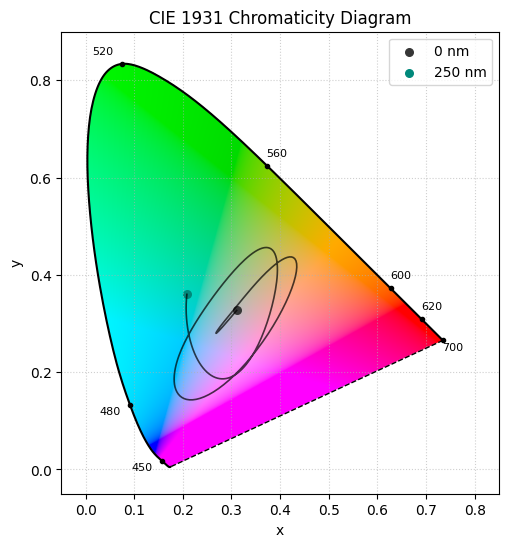

3) Plot the chromaticity path on the CIE 1931 diagram

Render the Michel-Levy color bar versus thickness

This compact color bar summarizes the perceived reflected color as a function of TiO_2 thickness. We obtain the Michel-Levy chart.

python

colors_array = be.asarray(colors)
colors_image = colors_array[None, :, :]

fig, ax = plt.subplots(figsize=(8, 1.6))
ax.imshow(
 colors_image,
 aspect="auto",
 extent=[float(thicknesses_nm[0]), float(thicknesses_nm[-1]), 0, 1],
)
ax.set_yticks([])
ax.set_xlabel("TiO2 thickness (nm)")
ax.set_title("Reflected color vs thickness")

plt.show()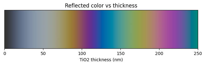

Show full code listing

python

import matplotlib.pyplot as plt
import optiland.backend as be
from optiland.materials import IdealMaterial, Material
from optiland.thin_film import SpectralAnalyzer, ThinFilmStack
from optiland.colorimetry.plotting import plot_cie_1931_chromaticity_diagram


air = IdealMaterial(n=1.0)
sio2 = Material("SiO2", reference="Gao")
tio2 = Material("TiO2", reference="Zhukovsky")

stack = ThinFilmStack(incident_material=air, substrate_material=sio2)
stack.add_layer_nm(tio2, 0.0, name="TiO2")

analyzer = SpectralAnalyzer(stack)

max_thickness_nm = 250.0
wavelengths_nm = be.linspace(380.0, 780.0, 81)
thicknesses_nm = be.linspace(0.0, max_thickness_nm, 251)

x_path = []
y_path = []
colors = []

for thickness_nm in thicknesses_nm:
  stack.layers[0].thickness_um = float(thickness_nm) / 1000.0

  result = analyzer.analyze_color(
      wavelength_values=wavelengths_nm,
      wavelength_unit="nm",
      aoi=0.0,
      aoi_unit="deg",
      polarization="u",
      quantity="R",
      observer="2deg",
  )

  x, y, _ = result["xyY"]
  r, g, b = result["sRGB"]

  x_path.append(x)
  y_path.append(y)
  colors.append([r / 255.0, g / 255.0, b / 255.0])

fig, ax = plot_cie_1931_chromaticity_diagram(color="fill")

ax.plot(x_path, y_path, color="black", linewidth=1.2, alpha=0.7)
ax.scatter(x_path[0], y_path[0], s=30, color=colors[0], label="0 nm")
ax.scatter(x_path[-1], y_path[-1], s=30, color=colors[-1], label="250 nm")
ax.legend()

plt.show()

colors_array = be.asarray(colors)
colors_image = colors_array[None, :, :]

fig, ax = plt.subplots(figsize=(8, 1.6))
ax.imshow(
  colors_image,
  aspect="auto",
  extent=[float(thicknesses_nm[0]), float(thicknesses_nm[-1]), 0, 1],
)
ax.set_yticks([])
ax.set_xlabel("TiO2 thickness (nm)")
ax.set_title("Reflected color vs thickness")

plt.show()

Conclusions

SpectralAnalyzer.analyze_color converts a raw reflectance spectrum directly into CIE XYZ tristimulus values, xyY chromaticity coordinates, and sRGB display values, bridging thin-film physics and human color perception in a single call.
Sweeping a TiO2 layer from 0 to 250 nm on a SiO2 substrate traces a curved path through the CIE 1931 chromaticity diagram, reproducing the classic thin-film color evolution (analogous to the Michel-Levy interference chart in mineralogy).
The 2-degree standard observer was used throughout, matching the photopic sensitivity of the human fovea and ensuring the computed colors are meaningful for display and visual inspection applications.
Accumulating sRGB triplets across the thickness sweep and rendering them as a 1D color bar provides an immediate visual reference — a designer can read off the perceived coating color directly from the layer thickness axis.
The same workflow generalizes to any single-layer or multilayer stack: substitute different materials or add more layers, and the chromaticity path and color bar update automatically without changing the analysis code.

Next tutorials

NextAnti-Reflective CoatingDesign broadband AR coatings to eliminate ghost reflections.RelatedThin-Film OptimizationRefine your coating designs to specific targets automatically.

Original notebook: Tutorial_6e_Color_Analysis_For_Thin_Film.ipynb on GitHub · ReadTheDocs