Catalogues

Thorlabs Catalogue

Directly import Thorlabs components from the web and analyze their sensitivity.

IntermediateLens Catalogue IntegrationNumPy backend12 min read

Introduction

This tutorial shows how to retrieve optical components from the Thorlabs lens catalogue. Building on the previous tutorial, we will show:

How to retrieve a lens model directly from the Thorlabs website
How to modify the lens properties after retrieval

Core concepts used

load_zemax_file(url)

Bypasses the download step by pulling the .zmx data directly from a web server into memory.

lens.updater.set_thickness

The low-level interface to modify any existing system property WITHOUT redefining the entire surface.

lens.image_solve()

A critical utility that automatically adjusts the last thickness (the air gap to the sensor) to find the 'best paraxial focus' of the system.

Step-by-step build

Import Required Libraries

python

import matplotlib.pyplot as plt
import numpy as np

from optiland import analysis
from optiland.fileio import load_zemax_file

Load Lens Directly from URL

File retrieval

As mentioned in the previous tutorial, the load_zemax_file function can accept either a Zemax (.zmx) file directly or a URL link to the file. Here, we will use the a Thorlabs Matched Achromatic Pair Lens and we will pass the URL directly to ZemaxFileReader. Optiland will download the file prior to reading the .zmx file.

python

# link to the .zmx file on Thorlabs website
url = "https://www.thorlabs.com/_sd.cfm?fileName=20565-S03.zmx&partNumber=MAP051950-A"

lens = load_zemax_file(url)

Draw the Imported Lens

We then draw the lens.

python

lens.draw()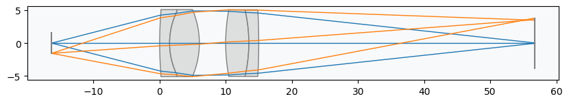

Inspect Lens Data

Let's print an overview of the lens data:

python

lens.info()

Generate Nominal Spot Diagram

Lens Analysis

Let's plot the nominal spot diagram:

python

spot = analysis.SpotDiagram(lens)
spot.view()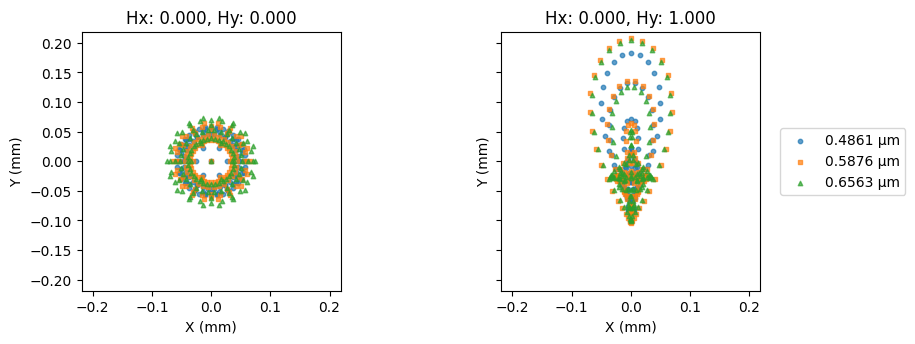

Sweep Object Plane Position

The lens is designed for finite conjugate applications. As an exercise, let's monitor the RMS spot size as a function of the object position. As we shift the object plane, we will reposition the image plane to the paraxial image location. We will use the on-axis field point (index=0) and the central wavelength (index=1).

python

# we will shift the object plane by ±3.0 mm from the nominal location
dz = np.linspace(-3.0, 3.0, 64)

# thickness between the object surface and the first lens surface
thickness = dz + 16.3412  # nominal location = 16.3412 mm

# set the wavelength and field indices
wavelength_idx = 1
field_idx = 0

# initialize variables
rms_spot_radius = []

for z in thickness:
 # change thickness on the first surface
 lens.updater.set_thickness(value=z, surface_number=0)

 # move image plane to maintain focus
 lens.image_solve()

 # generate spot diagram data
 spot = analysis.SpotDiagram(lens)

 # calculate RMS spot radius
 rms_spot_radius.append(spot.rms_spot_radius()[field_idx][wavelength_idx])

Plot RMS Spot Size vs. Object Shift

python

plt.plot(dz, rms_spot_radius)
plt.xlabel("Object plane shift (mm)")
plt.ylabel("RMS Spot Radius (mm)")
plt.title("RMS Spot Radius vs. Object Plane Shift")
plt.grid()
plt.show()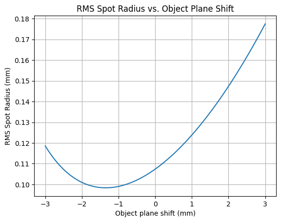

Show full code listing

python

import matplotlib.pyplot as plt
import numpy as np

from optiland import analysis
from optiland.fileio import load_zemax_file

# link to the .zmx file on Thorlabs website
url = "https://www.thorlabs.com/_sd.cfm?fileName=20565-S03.zmx&partNumber=MAP051950-A"

lens = load_zemax_file(url)

lens.draw()

lens.info()

spot = analysis.SpotDiagram(lens)
spot.view()

# we will shift the object plane by ±3.0 mm from the nominal location
dz = np.linspace(-3.0, 3.0, 64)

# thickness between the object surface and the first lens surface
thickness = dz + 16.3412  # nominal location = 16.3412 mm

# set the wavelength and field indices
wavelength_idx = 1
field_idx = 0

# initialize variables
rms_spot_radius = []

for z in thickness:
  # change thickness on the first surface
  lens.updater.set_thickness(value=z, surface_number=0)

  # move image plane to maintain focus
  lens.image_solve()

  # generate spot diagram data
  spot = analysis.SpotDiagram(lens)

  # calculate RMS spot radius
  rms_spot_radius.append(spot.rms_spot_radius()[field_idx][wavelength_idx])

plt.plot(dz, rms_spot_radius)
plt.xlabel("Object plane shift (mm)")
plt.ylabel("RMS Spot Radius (mm)")
plt.title("RMS Spot Radius vs. Object Plane Shift")
plt.grid()
plt.show()

Conclusions

This tutorial showed how to retrieve and analyze a Thorlabs catalogue lens.
We modified the lens properties and assessed the RMS spot size of the on-axis field as a function of the object plane shift. We compensated for the object shift by repositioning the image plane to the paraxial image location.

Next tutorials

NextCustom Surface TypesLearn how to define your own mathematical surface shapes in Python.RelatedEdmund Optics CatalogueA foundational look at local Zemax file importing.

Original notebook: Tutorial_9b_Thorlabs_Catalogue.ipynb on GitHub · ReadTheDocs