
Quickstart — Your First 5 Minutes#
This page takes you from a fresh install to a working, optimized optical system. Each section is self-contained: run any block in a Python script or Jupyter notebook.
1. Install#
pip install optiland
For GPU-accelerated differentiable ray tracing also install PyTorch:
pip install optiland[torch]           # CPU-only PyTorch
# or manually for CUDA:
pip install torch --index-url https://download.pytorch.org/whl/cu118
2. Hello, World#
Load and visualize a Cooke Triplet in 3D — two lines of code:
from optiland.samples.objectives import CookeTriplet

lens = CookeTriplet()
lens.draw3D()
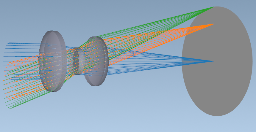
3D visualization of the Cooke Triplet lens system.#
Print the surface table (similar to a Lens Data Editor):
lens.info()
3. Build from Scratch#
Tip
The surface parameters below follow a specific model — see Conventions for why
thickness and material describe the space after a surface, not the surface itself.
Create a simple biconvex singlet in 8 lines:
from optiland import optic

lens = optic.Optic(name="Singlet")
lens.surfaces.add(index=0, radius=float("inf"), thickness=float("inf"))  # object at infinity
lens.surfaces.add(index=1, radius=50.0, thickness=5.0, material="N-BK7", is_stop=True)
lens.surfaces.add(index=2, radius=-50.0, thickness=0.0)
lens.surfaces.add(index=3)  # image plane
lens.set_aperture(aperture_type="EPD", value=10.0)
lens.fields.set_type("angle")
lens.fields.add(y=0.0)
lens.wavelengths.add(value=0.5876, is_primary=True)
lens.updater.image_solve()   # moves image surface to paraxial focus
4. Trace Rays#
Trace a bundle of rays and inspect the image-plane coordinates:
rays = lens.trace(Hx=0, Hy=0, wavelength=0.5876, num_rays=64, distribution="hexapolar")
print("x range:", rays.x.min(), "to", rays.x.max())
print("y range:", rays.y.min(), "to", rays.y.max())
Trace a single ray specified by normalized field and pupil coordinates:
# chief ray for the on-axis field
ray = lens.trace_generic(Hx=0, Hy=0, Px=0, Py=0, wavelength=0.5876)
5. Spot Diagram#
Visualize the geometric ray spread at the image plane:
from optiland.analysis import SpotDiagram

spot = SpotDiagram(lens)
spot.view()
The resulting plot shows the ray scatter for each field and wavelength. A tighter cluster indicates better image quality.
6. One-Step Optimization#
Minimize RMS spot size by varying two radii:
from optiland.optimization import OptimizationProblem, LeastSquares

problem = OptimizationProblem()
problem.add_variable(lens, "radius", surface_number=1)
problem.add_variable(lens, "radius", surface_number=2)
problem.add_operand(
    operand_type="rms_spot_size",
    target=0.0,
    weight=1,
    input_data={"optic": lens, "Hx": 0, "Hy": 0, "wavelength": 0.55,
                "distribution": "hexapolar", "num_rays": 6, "surface_number": -1},
)
optimizer = LeastSquares(problem)
result = optimizer.optimize()
print("Final merit:", result.cost)
7. Save and Load#
Serialize the optimized design to JSON and reload it in a new session:
from optiland.fileio import save_optiland_file, load_optiland_file

save_optiland_file(lens, "singlet.json")
lens2 = load_optiland_file("singlet.json")
lens2.info()
8. Beyond Imaging: Non-Sequential & Illumination#
Optiland also ships a differentiable non-sequential (NSQ) engine for illumination design, stray-light, and ghost analysis - where light is free to take any path through a 3-D scene. You can even convert an existing sequential lens in one line:
from optiland.nonsequential import sequential_to_nonsequential
scene = sequential_to_nonsequential(lens)
See the NSQ gallery overview and the on-ramp tutorial Tutorial 10a.
9. What Next?#
You have installed Optiland, built a lens, traced rays, run a spot diagram, optimized, and saved your design — all in under 5 minutes.
Choose where to go next based on your goals:
How Do I …? — a task-shaped index: find your question, get the notebook that answers it
Start Here — persona-based routing for students, engineers, researchers, and contributors
API Cheat Sheet — 20 copy-paste snippets for the most common tasks
Learning Guide — 60+ tutorials covering every feature in depth
Example Gallery — visual showcase of designs and analyses