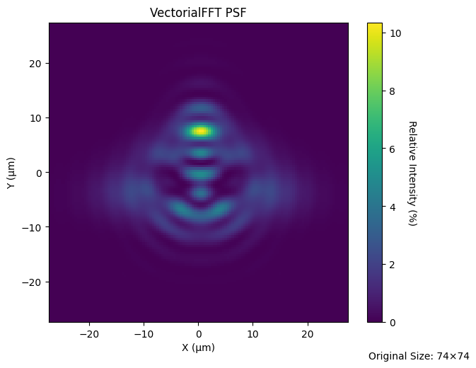
FFT Vectorial PSF - 2D

This example demonstrates how to use the VectorialFFTPSF class to calculate the 2D PSF of an optical system.

Note: Vectorial PSF calculations are automatically performed when polarization is enabled in the optical system. This accounts for the vectorial nature of the electric field at the exit pupil.

Method: For each ray, Optiland propagates the incident polarization state through the ray’s 3x3 polarization ray-trace (PRT) matrix to obtain the exit-pupil electric field, expressed in Cartesian (Ex, Ey, Ez) components. Each component is treated as an independent scalar pupil (same OPD-derived phase, different amplitude), 2D-FFT’d separately, and the resulting intensities are summed incoherently: |FFT(Ex)|² + |FFT(Ey)|² + |FFT(Ez)|². For unpolarized light, this sum also includes two orthogonal, incoherently superimposed input states. This is the discrete Fourier-optics analogue of the vectorial Debye-Wolf diffraction integral.

from optiland.psf import VectorialFFTPSF
from optiland.samples.objectives import CookeTriplet
from optiland.rays import PolarizationState

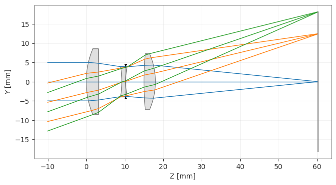
lens = CookeTriplet()
unpolarized_state = PolarizationState(is_polarized=False)
lens.updater.set_polarization(unpolarized_state)  # Enable polarization to trigger vectorial PSF
lens.draw()

(<Figure size 1000x400 with 1 Axes>, <Axes: xlabel='Z [mm]', ylabel='Y [mm]'>)

psf = VectorialFFTPSF(lens, field=(0, 1), wavelength=0.55)
_ = psf.view()