Optiland Torch Module - Custom Objective#
This notebook demonstrates a more advanced feature: defining a custom objective function. Instead of just minimizing RMS spot size, we’ll create a composite objective that simultaneously minimizes the spot size and penalizes the total length of the optical system. This showcases the flexibility of combining Optiland with PyTorch for complex design goals.
[1]:
import torch
import matplotlib.pyplot as plt
import optiland.backend as be
from optiland import optic, optimization
from optiland.ml import OpticalSystemModule
from optiland.wavefront import ZernikeOPD

be.set_backend("torch")  # Set the backend to PyTorch
be.grad_mode.enable()  # Enable gradient tracking
[2]:
lens = optic.Optic()
lens.surfaces.add(index=0, thickness=be.inf)
lens.surfaces.add(index=1, thickness=7, radius=200, material="N-SF11", is_stop=True)
lens.surfaces.add(index=2, thickness=50, radius=-200)
lens.surfaces.add(index=3)
lens.set_aperture(aperture_type="EPD", value=20)
lens.fields.set_type(field_type="angle")
lens.fields.add(y=0.0)
lens.wavelengths.add(value=0.55, is_primary=True)
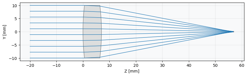
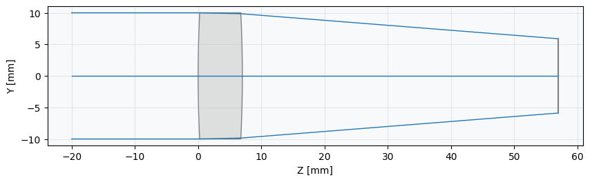
_ = lens.draw()
Build optimization problem#
First, we set up the standard optimization problem. We’ll define the RMS spot size as our primary operand and the lens radii as variables. The custom objective will build upon this foundation.
[3]:
problem = optimization.OptimizationProblem()
input_data = {
    "optic": lens,
    "surface_number": -1,
    "Hx": 0, "Hy": 0,
    "num_rays": 7,
    "wavelength": 0.55,
    "distribution": "hexapolar",
}
problem.add_operand("rms_spot_size", target=0, weight=1, input_data=input_data)
problem.add_variable(lens, "radius", surface_number=1)
problem.add_variable(lens, "radius", surface_number=2)
Define a Custom Objective Function
This is the core of this example. We create a Python function that returns our desired loss value. This function can perform any calculation using the underlying Optiland objects. Our objective will be:
where \(\lambda\) is a weighting factor to balance the two terms.
[4]:
def custom_objective():
    """
    Custom objective that minimizes both RMS spot size and total system length.
    """
    # Calculate the sum of squared errors from the optimization problem (our spot size term)
    spot_size_term = problem.sum_squared()

    # Add a penalty term proportional to the total length (total_track) of the lens
    # The 1e-3 factor balances the magnitude of the two terms in the loss function.
    length_penalty = 1e-3 * lens.total_track

    return spot_size_term + length_penalty
Define PyTorch module in Optiland#
We now pass our custom function to the OpticalSystemModule using the objective_fn argument. The module will call this function during its forward pass to compute the loss.
[5]:
model = OpticalSystemModule(lens, problem, objective_fn=custom_objective)
Define PyTorch Adam Optimizer and pass model parameters#
[6]:
optimizer = torch.optim.Adam(model.parameters(), lr=0.3)
Optimize with PyTorch#
[7]:
losses = []

for step in range(100):
    optimizer.zero_grad()         # Clear gradients
    loss = model()                # Forward pass computes RMS spot size
    loss.backward()               # Backward pass computes gradients
    optimizer.step()              # Update model parameters
    model.apply_bounds()          # Apply parameter bounds
    losses.append(loss.item())
[8]:
_ = lens.draw(num_rays=10)